دورة تدريبية عن تطبيقات برنامج ARC GIS

Transcription

1 دورة تدريبية عن تطبيقات برنامج ARC GIS مايو 2009

2 دورة تدريبيت عن تطبيقاث برنامج ARC GIS 2009 مايو

3 Table of Contents Introduction... viii Module 1: Introduction to ArcGIS 9 Module Objectives ArcGIS Desktop Software Suite Licenses Applications Basic Terms Common GIS Data Structures Spatial Data Types Supported by ArcGIS Vector Data Raster Data Tabular Data Metadata ArcCatalog Launch ArcCatalog Connect to a Folder Create a New Shapefile Preview an Existing Shapefile View Metadata ArcMap Launch ArcMap Add and Remove Data Layers The Map Document (*.mxd) The ArcMap Interface Data View and Layout View Coordinate Systems Data Frame Properties: Map Units Data Frame Properties: Display Units ArcToolbox Online Help Module 1 Exercise Module 1 Exercise i

4 Module 2: Displaying and Manipulating Spatial Information Module Objectives Map Scale and Zoom Tips Turning Data Layers On and Off Ordering Data Layers in the Table of Contents Layer Properties Set Display Units and Measure Distance on the Map Display Display an Attribute Table Sort Attribute Table Records Select Attribute Table Records Select Features Interactively Set Selection Options Set Selectable Layers Set Interactive Selection Method Select Individual Features from the Map Display Select Groups of Features from the Map Display Use the Identify Tool to See the Attributes of a Feature Map Tips Labels and Annotation Convert Labels to Annotation Display a Layer Based on Categorical Attribute Data Import an ArcView 3 Legend File (*.avl) Save a Layer File (*.lyr) Classify a Layer Based on Two Attributes Save a Map Document Module 2 Exercise ii

5 Module 3: Making A Thematic Map (Layout) Module Objectives Map Design Symbolizing Features Display a Layer Based on Quantitative Attribute Data Label Legend Classes Remove Symbol Outlines Save Your Work in a New Map Document Set a Reference Scale for a Data Frame Preparations for Creating a Layout Switch to Layout View Set the Layout Page Size and Orientation The Layout Toolbar Move and Resize a Data Frame in a Layout Manipulate Graphic Elements Insert a Title Insert a North Arrow Insert a Scale Bar Insert a Legend Insert Text Insert a Neatline Align Graphic Elements Create a Map Inset Symbolize a Map Inset Add a Data Frame Extent Rectangle to the Map Inset Add Graphics to a Data Frame from the Layout View Print a Layout Export a Map Map Templates Save a Layout as a Template NPS Map Templates and Graphic Identity Use an Existing Template Module 3 Exercise iii

6 Module 4: Selecting and Displaying Features Module Objectives Find Features Select by Attributes: Simple Queries Select by Attributes: Complex Queries Save and Load a Query Statement Show and Clear Selected Records in an Attribute Table Select by Location Export Selected Features Display a Subset of Features in a Layer: Using a Definition Query Module 4 Exercise Module 4 Exercise iv

7 Module 5: Displaying and Manipulating Attribute Data Module Objectives Components of an Attribute Table Change the Appearance of an Attribute Table Change the Width of a Field Freeze Fields in an Attribute Table Hide Fields in an Attribute Table Create an Alias for a Field Name Setting the Highlight Color for a Table Field Properties Field Type Field Length Precision and Scale View Statistics for a Field in an Attribute Table Summarize a Field in an Attribute Table Delete an Existing Field and Add a New Field to an Attribute Table Calculate Field Values Table Joins and Relates Join Data from One Table to Another Remove Joined Data Relate Data Between Two Tables Access Related Records Remove a Related Table Hyperlinks: Display Images of Spatial Features in a Data Layer Access a Feature s Hyperlink Module 5 Exercise Module 5 Exercise Mid-Term Exercise 2 v

8 Module 6: Other Data Types, Editing, Projecting, and Bookmarks Module Objectives Image Formats Add Image Data to a Map Document Heads-Up Digitizing Digitize Point Features Edit Data in an Attribute Table Digitize Polygon Features Digitize Line Features by Editing an Existing Shapefile Edit Vertices to Change the Shape of a Line Create a Point Layer from Tabular X/Y Data Create a Layer File (.lyr) from a Point Layer based on Tabular X/Y Data Project Data On-the-Fly Module 6 Exercise Module 7: Geoprocessing Module Objectives ArcGIS 9.1 Geoprocessing Tools Application Scenario Map Document Setup Merge Two Data Layers Buffer a Layer Clip A Layer Update Area and Perimeter Field Values Spatial Join Create a Summary Table Dissolve, Union, and Intersect Module 7 Exercise Module 7 Exercise Final Exercise: Fire Planning at Sequoia-Kings Canyon National Parks vi

9 Appendix A: Solutions to Exercises Module 1 Exercise 1... A-1 Module 1 Exercise 2... A-3 Module 2 Exercise... A-7 Module 3 Exercise... A-10 Mid-Term Exercise 1... A-11 Module 4 Exercise 1... A-15 Module 4 Exercise 2... A-18 Module 5 Exercise 1... A-23 Module 5 Exercise 2... A-25 Mid-Term Exercise 2... A-27 Module 6 Exercise... A-30 Module 7 Exercise 1... A-32 Module 7 Exercise 2... A-36 Final Exercise... A-39 vii

10 Introduction Required Software The purpose of this course is to teach you how to use ArcGIS software produced by Environmental Systems Research, Inc. (ESRI). For this course, you will need version 9.x of ESRI s ArcGIS software, i.e., ArcGIS 9.x, or ArcView 9.x. If you do not have version 9.x, you will not be able to open the map documents associated with the modules that comprise this course. Workbook Style Conventions The workbook has been designed to introduce a wide variety of GIS concepts and ArcGIS software-specific applications. Each module provides an overview of ArcGIS software functionality, specifies the objectives of the respective module, guides you through hands-on application scenarios, and provides one or more practical exercises. Throughout the workbook text in boldface type is meant to draw your attention to key terms, required processing steps, ArcGIS menus or dialog boxes, and pertinent file names. Representative screen captures are also included to provide guideposts throughout the materials. It s difficult to convey the entire breadth of the software s functionality in an introductory course so there are also many references to available on-line help and other sources of information to complement the provided materials. Mouse-Click Terminology Throughout the course workbook that follows, when you are instructed to: Click: Click once with the left mouse button. Double-click: Click twice in rapid succession with the left mouse button. Right-click: Click once with the right mouse button. viii

11 Glossary of GIS Terms You can access a glossary of GIS terms from ArcMap. Click on the Help menu item, then ArcGIS Desktop Help > Contents > GIS Dictionary (shown below). If you re migrating from an earlier version of ESRI s ArcGIS you may also want to review the What s new in ArcGIS Desktop 9.0 volume (see above). ix

12 Module 1

13 Introduction to ArcGIS for Module 1: Introduction to ArcGIS 9 A geographic information system (GIS) is a collection of hardware, software, geographic data, and personnel designed to create, store, edit, manipulate, analyze and display geographically referenced information. The purpose of this course is to teach you how to use ArcGIS software produced by Environmental Systems Research, Inc. (ESRI). For this course, you will need version 9.x of ESRI s ArcGIS software. Module Objectives When you have completed this module, you should understand: ArcGIS Desktop software suite licenses and applications Basic terms necessary to use ArcGIS Common GIS data structures Spatial data formats supported by ArcGIS How to navigate the primary ArcGIS Desktop applications: ArcCatalog and ArcMap How to use the ArcGIS Desktop Help system ArcGIS Desktop Software Suite Licenses ArcGIS Desktop is accessed using one of three software licenses with varying levels of functionality: 1. ArcView - provides comprehensive mapping and analysis tools with simple editing and geoprocessing capabilities 2. ArcEditor - provides all ArcView functions + advanced editing capabilities 3. ArcInfo - provides all ArcEditor functions + advanced geoprocessing and data management tools 1-1

14 Introduction to ArcGIS for Applications Regardless of license level whether ArcView, ArcEditor, or ArcInfo ArcGIS Desktop includes two main applications: ArcCatalog and ArcMap. ArcCatalog - used to organize and manage your GIS data. It also allows you to preview datasets and view and manage metadata. ArcMap - used to view, edit, and analyze spatial data and create maps. Editing functionality differs between license levels (ArcView, ArcEditor, ArcInfo). ArcToolbox was a separate application in ArcGIS 8.x, but is now a component of ArcCatalog and ArcMap. It contains tools for geoprocessing, data conversion, and defining map projections. The number and types of tools available in ArcToolbox differ between license levels (ArcView, ArcEditor, ArcInfo). The current release of ArcGIS is version 9.x. Versions of ArcGIS are not backward compatible, meaning that map documents created in version 9.x can NOT be used with earlier versions (e.g., version 8.x). However, this limitation is expected to be removed in version 9.1. As with most software, the versions ARE forward compatible. Map documents that you create in an earlier version (say 8.x) can be opened and manipulated in version 9.x. Basic Terms Point: a single location having an X, Y (and sometimes, a Z) position (point features have no area and no length) Line / Arc: a series of connecting X, Y positions (line features have length, but no area) Polygon: one or more connecting lines that form a single spatial feature (polygon features have both area and perimeter) Vertex: one of a set of ordered x,y coordinate pairs that define a line or polygon feature. More simply, a location along a line where the line changes direction giving it shape (similar to a point) Attribute Table: a table (much like a spreadsheet) that contains information about, and is linked to, spatial features. Each spatial feature has one associated record (row) in the attribute table 1-2

15 Introduction to ArcGIS for Common GIS Data Structures Vector: In a vector data structure, geographic features (such as wells, roads, national parks, etc.) are represented by points, lines, and polygons that are defined by a set or sets of [X,Y] coordinates. Raster: In a raster data structure, spatial data are stored in a two dimensional matrix, much like a checkerboard. Each raster, or cell, contains a value. Spatial Data Types Supported by ArcGIS The following data file types (i.e., data structures) are compatible with ArcGIS software. This is important information when you are requesting data from others. Vector Data ArcInfo Coverage - Topological layer, actually a collection of files in a directory that are linked to additional files found in the INFO directory. The INFO directory lives at the same level as the coverage directory. ArcView Shapefile - Non-topological layer, made up of at least three (and sometimes more) files with the following extensions,.shp,.shx, and.dbf ArcGIS Geodatabase A collection of feature datasets and classes--point, line, polygon--with topology (*.mdb extension) CADD datasets: Raster Data MicroStation design files (.dgn) AutoCAD drawing files (.dwg) and drawing interchange files (.dxf) Images DOQQ's, DRG's, with file extensions such as.tif,.bil,.jpg,.sid, etc. ArcInfo Grid - a raster data file analogous to an ArcInfo coverage, e.g., DEM s. Tabular Data Comma or tab delimited text (.txt) or dbase (.dbf) files containing coordinate data (X, Y coordinates) 1-3

16 Introduction to ArcGIS for Metadata Metadata, often referred to as data about data, describes the content, quality, condition and other characteristics of a geospatial dataset. The Federal Geographic Data Committee (FGDC) has adopted a content standard for metadata that all federal agencies are required to use to document newly created geospatial data. The FGDC content standard is a set of terms and definitions for documenting geospatial data and includes data elements organized under the following topics: Identification Information: basic information about the data set such as title, geographic area covered, date developed, stipulations regarding use of the data, etc. Data Quality Information: information about the quality of the data such as positional and attribute accuracy, data sources, methods used to produce the data, etc. Spatial Data Organization Information: information about the method used to represent spatial features in the dataset (e.g., raster, vector, street addresses, county codes, etc.) Spatial Reference Information: description of the reference frame for and method of encoding coordinate data including name of map projection or grid coordinate system, horizontal and vertical datums, and coordinate system resolution. Entity and Attribute Information: names and definitions of features, attributes, and attribute values contained in the dataset. Distribution Information: information about obtaining the dataset including name of distributor, available data format(s) and media, online availability, and fees. Metadata Reference Information: information on who prepared metadata and when. ArcCatalog ArcCatalog is the data management application of ArcGIS. ArcCatalog allows you to import, export, and preview datasets, drag and drop data to open ArcMap, and create feature class datasets and geodatabases. The Metadata function of ArcCatalog allows you to view, create, and/or edit metadata. Because spatial data may be composed of complicated file structures or multiple related files, it is important to use ArcCatalog rather than Windows Explorer to manage your data. With ArcCatalog, these complicated relationships are simplified and you can move, copy, or delete all related files with one operation rather than many. 1-4

17 Introduction to ArcGIS for The following exercise demonstrates how to use ArcCatalog to: Connect to a folder or directory Create a new shapefile Preview spatial data View metadata Launch ArcMap and open the ArcToolbox window Launch ArcCatalog 1. From the Start menu, select Programs > ArcGIS and click on the ArcCatalog icon. 2. When ArcCatalog opens, take time to hold the pointer over each of the buttons until the pop up label appears, displaying a short description of the button s function and a more detailed explanation in the status bar at the bottom of ArcCatalog. (Notice how similar the interface looks to that of Windows Explorer.) 3. In the directory tree on the left side, you see the various drives and folders on your computer, as well as other connection options (e.g., Database Connections, Address Locators, GIS Servers, etc.) You do not see all of the files and folders on your computer, instead you see only those folders to which a connection has been established. 1-5

18 Introduction to ArcGIS for Connect to a Folder In ArcCatalog, folder connections enable you to access your file-based data such as coverages, shapefiles, images, etc. All of the folder connections that you make are listed in the Catalog tree (see below). Once you have connected to a folder, you can browse its contents in the Catalog, including the contents of any of its subfolders. ArcCatalog allows you to connect to any folder on your hard drive as well as to folders on network drives. You may connect to the top level of a drive or to any subfolder. To improve efficiency, it is usually better to connect to subfolders rather than to the top level of drives. Think of folder connections as being like favorites. Make a separate connection to each of your most frequently used GIS folders. In this way, you will have the most convenient access to your data because you will not have to click down through a series of subfolders to get to it. Now, connect to the folder where the files for this course are saved, as follows: 1. Click on the Connect to Folder icon in the menu bar. 1-6

19 Introduction to ArcGIS for 2. Navigate to the folder where the data for Module 1 of this course are saved (e.g., \nps_agis9\module1\data) in the Connect to Folder dialog. 3. Click OK. The \nps_agis9\module1\data folder now appears in the Catalog tree. To remove a folder connection, right-click on the folder path\name in the Catalog tree and select Disconnect Folder from the context menu that appears. Create a New Shapefile Like creating a New Folder in windows, feature classes such as shapefiles can be created in ArcCatalog. Make sure the \nps_agis9\module1\data folder is selected or highlighted. 1. Click on File in the Menu Bar and choose New > Shapefile. 1-7

20 Introduction to ArcGIS for 2. The Create New Shapefile dialog window opens. Name the new shapefile nps_example and choose the Polygon Feature Type from the dropdown menu. 3. Spatial Reference refers to the coordinate system in which the data are to be stored or projected. Click the Edit button in the Create New Shapefile dialog then click the Select button in the Spatial Reference Properties window. 4. Double-click on the Projected Coordinate Systems folder and then on the State Plane folder. The folders containing North American Datum (NAD) are now displayed in the Browse for Coordinate System window. 5. Double-click on the NAD 1983 (Feet) folder and navigate to the NAD 1983 State Plane North Carolina FIPS 3200 (Feet).prj file. 6. Select the file and click Add. The Coordinate system is now displayed in the Spatial Reference Properties window. 7. Click OK and view the Spatial Reference Description in the Create New Shapefile dialog. 1-8

21 Introduction to ArcGIS for 8. Click OK and notice the new shapefile in the \nps_agis9\module1\data folder. Preview an Existing Shapefile 1. In the Catalog Tree on the left side of the ArcCatalog window, navigate to \nps_agis9\module1\data\anjo\shpfiles. Click on the anjo_boundary.shp shapefile in the catalog tree on the left side of the ArcCatalog window. Select the Contents tab and you will see a polygon icon, indicating that this shapefile contains polygon features. 2. Select the Preview tab to preview the contents of this shapefile 3. At the bottom of the Preview area, click on the dropdown arrow to the right of the small window labeled Preview: and choose Table. This allows you to view the shapefile s attribute table. 1-9

22 Introduction to ArcGIS for View Metadata The next tab is used to view Metadata. 1. Select the Metadata tab. The metadata for the anjo_boundary.shp file is now displayed. Notice that the Metadata toolbar becomes active. 2. Hold the pointer over each Metadata button to see its function. 3. Change the stylesheet from FGDC ESRI to FGDC by clicking on the Stylesheet dropdown list and selecting FGDC. Notice that there are links to each of the major sections of the metadata record located just below the FGDC and ESRI Metadata: heading. (You may need to scroll down slightly to see these links.) For example, click on the link for Spatial Reference Information. This section of the metadata record contains important information about the coordinate system in which these data are projected. ArcMap ArcMap is the ArcGIS application that you use to display, query, edit, create, and analyze geographic data. Launch ArcMap ArcMap can be launched independently or from ArcCatalog. Use one of the following methods to launch ArcMap with A new empty map now: 1. You may launch ArcMap by clicking Start > Programs > ArcGIS > ArcMap. When prompted, select A new empty map. 2. To launch ArcMap from ArcCatalog, click on the ArcMap icon on the standard toolbar. ArcMap will take a moment to open. When prompted, select A new empty map. Add and Remove Data Layers To illustrate basic features of the ArcMap interface, add a shapefile and a TIF image to your new empty ArcMap map document, as follows: 1-10

23 Introduction to ArcGIS for 1. If necessary, turn on the Standard Toolbar by clicking on the View menu item > Toolbars > Standard. 2. Click the Add Data button on the standard toolbar. In the Add Data dialog, navigate to \nps_agis9\module1\data\anjo\shpfiles folder, highlight anjo_boundary.shp, and click the Add button. Notice that the data layer, anjo_boundary, is added to the Layers data frame in the ArcMap Table of Contents. 3. Use the same procedures to add a DOQQ, GREENEVILLE_SW.tif located in \nps_agis9\module1\data\anjo\doqs, to your map. For now, click OK to bypass the Spatial Reference warning window that pops up. 4. To remove a data layer, right-click on the name of the layer in the Table of Contents window and select Remove from the context menu that appears. The Map Document (*.mxd) A map document (which has an.mxd file extension) is the fundamental component you work with in ArcMap. A map document is a collection of data layers and cartographic layouts. Map documents store references to the locations of the data sources (e.g., shapefiles, coverages, image files, etc) NOT the data themselves. Save your untitled map document, as follows: 1. Click File in the menu bar and select Save from the dropdown list. 2. In the Save dialog, navigate to the folder in which you want to save your map document (e.g. \nps_agis9\module1). 3. Type in a file name, anjo, and click the Save button. Notice that the file name anjo.mxd now appears in the ArcMap title bar. The ArcMap Interface Key components of the ArcMap interface are: The title bar, menu bar, and toolbars; Two side-by-side windows: the Table of Contents and the map display window; The status bar. The Title Bar at the top of the ArcMap window displays the name of the map document. 1-11

24 Introduction to ArcGIS for The Menu Bar, located just below the Title Bar contains a series of menu items: File, Edit, View, Insert, Selection, Tools, Window, and Help. Clicking on a menu item opens a dropdown menu with numerous options. To select an option on the dropdown menu, click and release the mouse button on the option. ArcMap includes a variety of Toolbars. Click on the View menu item and select Toolbars to see all of the toolbars that are available to you. A check mark next to the toolbar name indicates that it is visible. For now, be sure that the Standard Toolbar and the Tools Toolbar are turned on, as shown below: The Standard Toolbar contains buttons that give you fast and easy access to many of the Menu Bar options. Click on the button to execute a particular operation. The Tools Toolbar includes tools that allow you to interact with the data displayed in the map display window to carry out specific tasks. Typically, the pointer changes when a tool is used. 1-12

25 Introduction to ArcGIS for ArcMap provides a number of other toolbars, such as: Draw - for drawing graphics and adding text Editor for editing spatial data Layout for working with layouts Effects for altering the display of spatial data Take a look at these and some of the other toolbars and their tools. You can access the toolbars list without using the View menu by right-clicking any toolbar or the status bar. To quickly hide or turn off a toolbar, click its Close button. The Status Bar, located at the bottom of the ArcMap window, gives you information about the function of a button or a tool when you hold the pointer over it. The status bar also displays the coordinate position of the mouse pointer in the display window and information about the progress of particular operations, e.g., printing a layout. The Table of Contents, located on the left side of the ArcMap window, lists all of the layers that you have added to your map and shows the symbols that are used to represent the features in each data layer. The check box next to each layer name indicates whether it is currently displayed in the map display window to the right of the Table of Contents (i.e., whether it is turned on or turned off.) The order of layers within the Table of Contents is important because the layers at the top draw on top of those that are listed below them. At the bottom of the Table of Contents there is a Display tab, a Source tab, and a Selection tab. When you select the Display tab, you see the drawing order of the layers and you can move a layer up or down in the Table of Contents by dragging and dropping it. 1-13

26 Introduction to ArcGIS for 1. Move the anjo_boundary layer to the bottom of the Table of Contents and notice what happens. 2. Now, move it back to the top of the Table of Contents. When you select the Source tab, layers are sorted by where they are stored on disk. This is useful during editing when you want to edit all layers in a given folder or database. You cannot change the drawing order of layers when the Source tab is selected. The Selection tab allows you to choose the layers from which features can be selected. This function is described using a different method in Module 2. Within the Table of Contents, data layers that you add to your map are grouped into one or more data frames. A data frame is a group of data layers that you want to display together. When you create a map or map document in ArcMap, it always contains at least one data frame, with the default name of Layers that is listed at the top of the Table of Contents. You can change the data frame name to something more meaningful. In ArcMap, geographic information is displayed on a map as layers. Each data layer represents a specific type of feature such as rivers, lakes, archaeological sites, political boundaries, etc. A data layer does not store the actual geographic data; instead, it references the data contained in coverages, shapefiles, geodatabases, images, grids, and so on. Referencing data in this way allows the layers on a map to automatically reflect the most upto-date information in your GIS database. Data View and Layout View ArcMap provides two different ways to view a map: data view and layout view. Use data view when you want to browse, edit, and/or analyze the geographic data on your map. Layout view is used to prepare finished maps for printing and publication. (You will learn more about layouts in Module 3.) To switch between data and layout views: 1. Click the View menu item and select either Data View or Layout View from the context menu that appears. 2. Alternatively, you can use the Data View and Layout View buttons located in the lower left portion of the view window to switch between these two views. 3. When you switch to Layout View, the Layout toolbar is automatically added to the ArcMap window. These tools allow you to zoom in and out, pan, and zoom to set extents (e.g. full page, 1:1) on the layout. 1-14

27 Introduction to ArcGIS for Coordinate Systems Spatial data are data that are georeferenced. That is, they are referenced to the surface of the earth using either a geographic coordinate system or a Cartesian (projected) coordinate system. Geographic coordinate systems use latitude and longitude for coordinates. Even though only two coordinates are required to locate a point on the earth s surface, latitude/longitude are three-dimensional coordinates because the earth s surface is threedimensional. Projected coordinate systems use a mathematical conversion to transform latitude and longitude coordinates that fall on the earth s three-dimensional surface to a flat two-dimensional surface. A projected coordinate system is made up of a spheroid, datum, projection, and horizontal units (i.e. map units). ArcGIS can work with data stored in either geographic or projected coordinates. Data Frame Properties: Map Units Map units are the horizontal measures (feet, meters, etc) in which distances are calculated in a data frame. They are different from the Display units, which are the horizontal measures in which distances are actually displayed on the screen. For example, you might be using data stored in State Plane feet (so the map units are set to feet), but making distance measurements in meters (the display units). Map units are set when a coordinate system is selected for a data frame. The data frame coordinate system is automatically set to the coordinates of the first data layer added to the data frame. This feature is very useful when data stored in different coordinate systems are going to be used together. For example, you might want to display a data layer with UTM coordinates on top of a layer stored in latitude/longitude. ArcGIS reprojects the data on-thefly to whatever coordinate system is specified for the data frame. The map units cannot be altered by the user in this situation. However, on-the-fly projection does not work correctly unless all the data layers in a data frame have their coordinate systems defined -- usually in a projection file with a.prj extension. If you add a layer that does not have a defined coordinate system, ArcMap displays a warning message: "One or more layers is missing spatial reference information. Data from those layers cannot be projected." (On-the-fly projection will be covered in more detail in Module 6.) 1-15

28 Introduction to ArcGIS for Finally, if a data frame does not have a selected coordinate system (probably because the first added data layer didn't have a prj file), then the map units should be set by the user to whatever coordinate system is appropriate for the data in the data frame. In this case, all data layers should be stored in the same coordinates; otherwise serious misalignment issues can arise. Your ArcMap map document, anjo.mxd, currently contains one data frame, named Layers, and two data layers. The first data layer that you added, anjo_boundary, is a shapefile that includes a projection file (anjo_boundary.prj). Because the anjo_boundary shapefile includes a projection file, when you added it to your map document, ArcMap set the data frame s coordinate system and map units based on information in the projection file. 1-16

29 Introduction to ArcGIS for 1. Right-click on the data frame name Layers and select Properties from the context menu that appears (shown below). 1-17

30 Introduction to ArcGIS for 2. Click on the General tab in the Data Frame Properties dialog and notice that the map units are set to feet and that this control is disabled. 1-18

31 Introduction to ArcGIS for 3. Click on the Coordinate System tab and notice that the coordinate system has also been set. Cancel out of the Data Frame Properties dialog when you have finished examining its contents. Data Frame Properties: Display Units Display units are used to report measurements you make using the measure tool, dimensions of shapes, distance tolerances, and offsets. Using the Data Frame Properties dialog, you may set display units to any unit of measure that is convenient or necessary for a specific task. Display units are independent of map units. Note: Map and Display units will be covered in more detail in the next module. 1-19

32 Introduction to ArcGIS for ArcToolbox The ArcToolbox Window contains tools for manipulating geospatial data and is organized into toolboxes. The four main toolboxes we ll examine are: Analysis Tools for performing geoprocessing functions. Conversion Tools allow the import and export of geospatial data and other data formats compatible with ArcGIS. Data Management Tools used to develop, manage, and maintain feature classes, datasets, layers and raster data structures. Geoprocessing Wizard Tools contains the most commonly-used analytical tools, which you ll use in Module 7. Toolboxes contain toolsets and tools. Toolsets are used to group collections of tools together into logical groupings. A tool is an entity that performs a specific geoprocessing task such as generalizing lines. There are three types of tools: System tools let you analyze and modify spatial data. Models run a chain of tools in sequence. Scripts take advantage of the command line to run tools in sequence and are useful for batch processing-for example, converting many datasets to another format or running the same model with a series of different input datasets. Use the ArcToolbox icon in ArcCatalog or ArcMap to open the ArcToolbox Window. This will add a new frame to the main ArcCatalog or ArcMap interface. Navigate through the ArcToolbox toolboxes to familiarize yourself with the tools available. When you are finished, close the ArcToolbox Window. 1-20

33 Introduction to ArcGIS for Online Help The help system in ArcGIS contains a wealth of information it is well worth your time to learn how to access this information. Help can be accessed in a variety of ways. 1. Context Sensitive Help can be accessed with the What s This? Button, on the standard toolbar: Click on the button then click a menu item, button or tool to see the definition or purpose of it, as shown below. 1-21

34 Introduction to ArcGIS for 2. Clicking on the Help menu item gives you access to the complete ArcGIS Desktop Help system. The ArcGIS Desktop Help window has four tabs: Contents, Index, Search, and Favorites. The help documents are organized by topic and often by application, that is ArcCatalog, ArcMap, etc. 1-22

35 Introduction to ArcGIS for 3. You can also press the F1 key to access help about dialog box controls. Place the pointer over an item and press the F1 key. Take time to become familiar with each of these methods of accessing help information. It is also wise to observe patterns in what help routines take what amounts of time to access, which ones are less functional when other software is open, etc. 1-23

36 Introduction to ArcGIS for Module 1 Exercise 1 There is a major project within the NPS GIS community to bring digital versions of the NPS Land Status maps into each park s standard GIS database. A significant aspect of this project is to digitally check the geopositioning of each of the scanned park boundary and tract maps with a reference source. The standard reference source is a USGS Digital Ortho Quarter Quad (DOQQ) image mosaic, which is usually a layer in the base cartography data set available for each natural resource-based Inventory and Monitoring park. In this exercise you are the Resource Manager at De Soto National Memorial. You have been asked to verify that the contractor produced shapefiles for the park boundary and tracts line up with the park s DOQQs. The product is a report describing the consistency of the shapefiles with the DOQQs. The shapefiles and the DOQQ mosaic are located in the \nps_agis9\module1\data\deso\ folders. One objective of this exercise is to continue exploring display capabilities within ArcMap. Hint: Since this is your first exercise you get a little extra help! 1. Open a new empty map in ArcMap and use the Add Data button to add the DOQQ mosaic and shapefile layers. 2. Use the Connect to Folder button in the Add Data dialog to establish a connection to the folder where data for this exercise are stored (e.g., \nps_agis9\module1\data\deso\), then add the image and shapefile data, both Boundary and Tracts. Make sure that the DOQQ mosaic is at the bottom of the Table of Contents. 3. Change the draw order of the two shapefiles, and see if you can figure out how to display them without a fill color to make it easier to inspect their alignment with the DOQQ. 4. Right-click on Boundary and select Zoom to Layer. Now that you can clearly see the Boundary and Tract layers superimposed on the DOQQ, can you tell whether the contractors did a solid job of matching the shapefile to the DOQQ? (Inspect the shoreline, in particular.) Also, do the Tracts and Boundary layers line up well? 1-24

37 Introduction to ArcGIS for Module 1 Exercise 2 Use ArcGIS Desktop Help, including the GIS Dictionary, to answer the following questions: 1. How are Save and Save As different? 2. Define Metadata. 3. How do you edit metadata in ArcCatalog? 4. How do you add data to the data frame? 5. How do you print a map displayed in ArcMap? 6. What is the importance of specifying map units in an ArcMap document? 7. What ArcGIS application would you use to determine the projection of an image, shapefile, or coverage? 1-25

38 Module 2

39 Module 2: Displaying and Manipulating Spatial Information In ArcGIS, geographic features (such as cities, counties, roads, streams, etc.) are represented by points, lines, and polygons that are defined by a pair or pairs of X, Y coordinates. One of the defining characteristics of a GIS is that information about geographic features (i.e. attributes) are linked to the points, lines, and polygons representing the features so you can select and manipulate features based on their attributes. For example, with the appropriate data, you can select all of the roads above a specified width and display them in a different color or with a different symbol than narrower roads. Or, you can identify what types of land use occur within a specified distance of a historic structure or some other selected feature. Module Objectives In this module you will learn how to: Manipulate the appearance of spatial displays Display, sort, and select attribute data Select spatial features and display their attributes Label features Display layers based on categorical attributes Import an ArcView 3 legend file Save a layer file Map Scale and Zoom Tips Map scale is the relationship between distance measured on a map and the corresponding realworld distance. The simplest way to describe a map s scale is with a representative fraction or a ratio in which the numerator, representing map distance, is always 1 and the denominator represents the corresponding distance on the ground. A map scale of 1/24,000 or 1:24,000 means that one unit of measure on the map equals 24,000 of the same units on the earth. Other methods of indicating map scale are descriptive statements such as 0.5 inch = 2 miles or 0.5 inches to the mile and graphic scales or scale bars which look like a small ruler printed on the map. 2-1

40 In ArcGIS, you can change the scale at which your data are displayed as long as the map units are set correctly. You can enter a scale in the map scale box display will automatically be updated by ArcMap. and the map 1. Launch ArcMap and open the map document, SHILOH.mxd, found in the \nps_agis9\module2 folder 2. Notice that the scale box is in gray and cannot be changed. This is because the Map Units have not been set for this map document. 3. Right click on the Park View data frame, and choose Properties. Under the General tab of the Data Frame Properties window, notice that the Map Units are set to Unknown Units. Click on the dropdown list, and choose Meters. Click OK to close the Data Frame Properties window. 2-2

41 4. In the map scale box on the Standard toolbar (under the menu bar at the top of the ArcMap window) enter to display the Shiloh map at a scale of 1:24,000, as follows: 5. Try entering different scales and notice that the map display zooms in or out depending on the scale you enter. This function now works because the Map Units are set correctly. Brain Teaser: What happens if the Map Units are set incorrectly say, to inches? When you use the zoom tools to zoom in or zoom out on the map display, you are actually changing the scale of the map. Zooming in (making the scale larger) allows you to see more 2-3

42 detail and zooming out (making the scale smaller) allows you to view a bigger area but in less detail. Use the tools in the Tools toolbar (illustrated below) to practice zooming in and out on the Shiloh map display. 1. Explore the effect of the Fixed Zoom In and Fixed Zoom Out buttons located on the toolbar. 2. Try the Zoom To Full Extent button found on the toolbar. 3. Experiment with the Zoom to Layer by right-clicking on the name of a data layer in the Table of Contents and choosing this icon. 4. Experiment with the Go Back to Previous Extent and Go to Next Extent buttons found on the toolbar. 5. Experiment with the Zoom In, Zoom Out, and Pan tools found on the toolbar. Use the zoom tools to drag a box around an area of interest. Turning Data Layers On and Off 1. Zoom to the extent of the Shiloh NMP layer 2. Make sure that the Streams and Lakes layers are displayed on your map. To display a layer, turn it on by clicking on the check box to the left of the layer name in the Table of Contents. Note: A layer is On (visible) if the layer has a check mark in the box to the left of the layer name. 2-4

43 Ordering Data Layers in the Table of Contents As you learned in Module 1, the order of layers in the Table of Contents is important because layers at the top draw on top of those that are listed below them. When the Display tab (located at the bottom of the Table of Contents) is selected, layers are shown in the order in which they will be drawn and you can move a layer up or down in the list. (You cannot change the drawing order of layers when the Source or Selection tabs are selected.) 1. Make sure the Display tab is selected at the bottom of the Table of Contents. 2. Click and Hold on the Vegetation layer name and drag it to the top of the Table of Contents. 3. Click and Hold on the Vegetation layer name and drag it to the bottom of the Table of Contents. Notice that when you put the Vegetation layer at the top of the Table of Contents, all the other points, lines, and polygons are covered by the vegetation polygons. It is usually a good idea to place point layers at the top of the Table of Contents, then line layers, and finally, place polygon layers at the bottom of the Table of Contents. (This is the default order when adding layers using the Add Data button in ArcMap.) 2-5

44 Layer Properties The Layer Properties dialog allows you to view and/or control all aspects of a layer such as: How to draw or symbolize the layer How to display selected features What data source the layer is based on Whether and how to label the layer s features Attribute field properties What data are joined or linked to the layer For example to display and manipulate the properties of the Survey Plots layer: 1. Right-click the layer name, Survey Plots, in the Table of Contents and select Properties from the context menu that appears. (You can also double-click a layer name in the Table of Contents to display its Layer Properties dialog.) 2-6

45 2. Click the General tab. Notice that you can change the name of the layer, turn the layer on or off, and set a map scale above or below which this layer will not be shown. 3. Click the Source tab to view information about the source data. Notice the Set Data Source button that allows you to redirect a layer to another data source. This is particularly useful when a data source has been moved from its original location. 4. Options under the Selection tab allow you to specify a symbol and/or color for displaying selected features 5. The Symbology tab is used to control classification and display of the layer s features. (We illustrate how to classify a layer later in this module.) 6. Click the Fields tab to see the name, type, length, precision, and scale of each attribute (field) in the layer s attribute table. 7. Click each of the other tabs to view or manipulate other layer properties. When you are finished, close the Layer Properties dialog. 2-7

46 Set Display Units and Measure Distance on the Map Display In ArcMap, you can measure the distance between two points using the measure tool located on the standard toolbar. Display Units is the data frame property that controls what measurement unit is used to report distance measurements. The following steps illustrate how to set display units for a data frame and then how to use the measure tool to measure the distance between two points on the map display. 1. First, you will set the Display Units for the Park View data frame. Right-click on the Park View data frame name at the top of the Table of Contents. 2. Choose Properties at the bottom of the context menu. 3. Under the General Tab, note that Map Units are set to Meters and Display Units are set to Unknown Units. Note: As was explained in Module 1, map units must be set to the measurement units in which the data are stored or projected (e.g. UTM-17, NAD83, meters). 4. Change the Display Units by selecting Feet from the dropdown list. Click OK. 2-8

47 5. Select the Measure tool from the toolbar to measure the distance between two Survey Plots. 2-9

48 6. Click once on a Survey Plot then double-click on another Survey Plot. (Note that you cannot snap to the survey plots.) 7. Look at the left side of the Status bar at the bottom of the window to see the distance, in feet, between the two survey plots. Note: the numbers in the right-hand portion of the Status Bar indicate the coordinate location of the cursor in display units. Move the cursor and you will see these numbers change. Be sure you are looking at the correct numbers to read the results of your measurement. 8. Try setting the Display Units to meters and then measure the distance between two other survey plots. 2-10

49 Display an Attribute Table 1. Make sure the Vegetation layer is turned on and that it is placed at the bottom of the Table of Contents. Right-click the layer name in the Table of Contents. 2. From the context menu that opens, choose the Open Attribute Table option. 3. Use the scroll bars on the right and bottom of the table window to scroll through the fields and records in the table. Notice the caption at the bottom of the table, Records (0 out of 359 Selected) this table contains a total of 359 records. 2-11

50 Sort Attribute Table Records 1. In the Attributes of Vegetation table, right-click on the heading for the field (column) named CLASS. The following menu containing options for manipulating data in the table appears: 2. From this menu click the Sort Ascending button. Notice the records in the table are now sorted in alphabetical order according to the values in the CLASS field, allowing you to find records with a specific class value more easily. 3. Try the Sort Descending button with the Area field and notice how the records are sorted. Select Attribute Table Records 1. Use the Select Elements tool to click the leftmost field in the table adjacent to the record you want to select (the gray box to the left of the first field). ArcMap highlights both the selected table record and the feature associated with that record in the map display, as shown below. 2-12

51 2. Hold down the <Ctrl> key and select a few additional records. To select consecutive records, click on the first record and drag the cursor down the field until you reach the last record you wish to select. Notice that updated information regarding number of records selected is displayed at the bottom of the table window. 3. To clear or unselect the records, click on the Options button in the bottom right of the table window and then select Clear Selection (as shown below). Then select a few records and click on Switch Selection a few times to see what happens. 2-13

52 4. If you wish to unselect selected records in all layers, click on the Selection menu item in the menu bar and choose Clear Selected Features (as shown below). This will unselect all selected features, and consequently all selected records, in all layers. 5. Close the Attributes of Vegetation table. Select Features Interactively ArcMap provides a couple of different ways to select features interactively (i.e., directly from the map display). However, before you begin selecting features, you should set appropriate parameters to insure that you select the features that you think you are selecting and to increase the efficiency of the selection process. These parameters include a set of selection options, selectable layers, and selection method. 2-14

53 Set Selection Options To open the Selection Options dialog, click on the Selection menu item and then on Options. The Selections Options dialog should look like this: Take a look at each of the headings and individual parameters that you can set using the Selection Options dialog. For now, you do not need to change any of the default settings. Click Cancel to close the Selection Options dialog. 2-15

54 Set Selectable Layers 1. Click the Selection menu item at the top of the ArcMap window and then choose Set Selectable Layers. 2-16

55 2. Click the Clear All button to unselect all layers. 3. Click the box to the left of the Vegetation layer name (which makes the Vegetation layer selectable) and then click Close. You can also set selectable layers in the Selection tab in the Table of Contents 2-17

56 Set Interactive Selection Method 1. Click the Selection menu item and then click Interactive Selection Method, as follows: 2. For this example, we want to create a new selection, so you do not need to alter the default setting. However, you should be aware of the other selection method options that are available. Select Individual Features from the Map Display 1. Zoom in so that you can easily see the boundaries between vegetation polygons on the map display. 2. Click on the Select Features tool in the Tools toolbar. When you move the cursor to the map display it will look like this:. 3. Click on a vegetation polygon. To select more than one vegetation polygon, hold down the <Shift> key and click on additional polygons. 4. Select two or more vegetation polygons on the map display. 5. Now, open the attribute table for the Vegetation layer: right-click on the Vegetation layer name in the Table of Contents and select Open Attribute Table. The dialog at the bottom of the window shows the number of Records selected. 2-18

57 6. Press the Selected button next to the Record count. 7. A new window, Selected Attributes of Vegetation, opens displaying only the selected records. Press the All button at the bottom of this window to redisplay all the records. 8. Use the Selection menu item to unselect all records (Clear Selected Features). 9. Close the Attributes of Vegetation table. 2-19

58 Select Groups of Features from the Map Display There are two ways to interactively select groups of features from the map display in ArcMap. You can use the Select Features tool to drag a box around multiple features to select all the features within or intersecting that box (depending on the interactive selection setting you selected in the Selection Options dialog). Alternatively, you can draw a graphic around features and use the Select by Graphics option. 1. First, turn off all layers except the Survey Plots and Shiloh NMP layers. Right-click on the Shiloh NMP layer and select Zoom To Layer to display the full extent of this layer and center it on the screen. 2. Make Survey Plots the only selectable layer. Your data display should now look like this: 2-20

59 3. Click on the Select Features tool. Click and drag a rectangle around the survey plots in the northern half of the park. When you release the cursor button, the survey plots inside the rectangle that you formed with the cursor are selected. 4. Clear the selected features. 5. To use the Select By Graphics method, you must first draw a graphic around the features you wish to select. If it is not already enabled, turn the Draw toolbar on. Click the dropdown arrow to the right of the Draw a rectangle button and select the New Polygon icon, as shown below: 2-21

60 6. Move the cursor to the map display and draw a polygon that encloses several survey plots. When you close the polygon, it will probably display with a fill that obscures the survey plots. When you remove the polygon graphic (in step 8) after performing the selection, the features will be selected. Click on the Selection menu item and then on Select By Graphics. In the map display, you will see the selected features inside the graphic you drew, as illustrated below. A second option to enable viewing of the plots is to remove the fill color of the polygon. Right-click inside the polygon graphic and select Properties, then select the Symbol tab and Fill color. Choose No color and the selected point features become visible. 2-22

61 7. Open the attribute table for the Survey Plots layer and click the Selected button below the table to see the records that are selected. 8. Close the Attributes of Survey Plots table, clear selected features, and delete the polygon graphic. (To delete the graphic, select it with the Select Elements tool and press the <Delete> key.) Use the Identify Tool to See the Attributes of a Feature 1. Turn on the Lakes layer. 2. Click on the Identify tool located on the Tools toolbar. The Identify Results window opens and the appearance of the cursor changes; the cursor should now look like this:. When you click on a tool, you change the function of the cursor and interact directly with the features in the map display area. 3. Using the Identify tool click on a lake to see its attribute information. The Identify Results window displays the attribute data associated with the feature. 2-23

62 By default the Identify Results window displays the attributes of the feature in the <Topmost layer>. If you want to view the attributes of a feature in a different layer, use the dropdown list of Layers located at the top of the window to choose the appropriate layer. 4. Close the Identify Results window. Map Tips Map tips provide interactive access to information about map features. The way this works is that you define an attribute field that will pop up when you pause the mouse pointer over a feature in the ArcMap data display window. This is a quick way to see the name of a feature or some other piece of information about it without having to use the Identify tool. 1. In the Table of Contents, right-click the Survey Plots layer name and then click Properties from the context menu that appears. 2. In the Layer Properties dialog, click the Display tab and then check the Show Map Tips box at the top of the Layer Properties dialog, as follows: 2-24

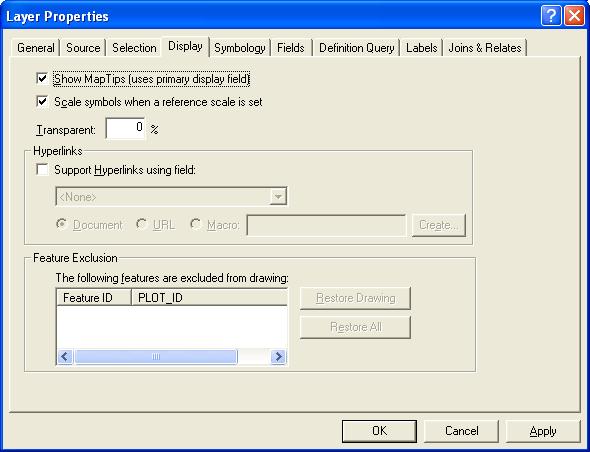
63 2-25

64 3. Click the Fields tab. 4. Click the Primary Display Field dropdown arrow and select the PLOT_NUM attribute field. 5. Click OK. 6. Move the mouse pointer over a plot in the data view map display to see the map tip. Labels and Annotation Labels and annotation are the two main kinds of text that ArcGIS supports. In ArcMap, labels are placed dynamically and provide a quick and easy way to add descriptive text for many features based on their attributes. Annotation is used to add descriptive text for a few features or to add text that is not associated with a specific feature. You can label the features in a data layer with any of the attribute values stored in the attribute table. In the following example, you will label each point in the Survey Plots layer with its plot number. In the attribute table for this data layer, the field named PLOT_NUM contains the plot number for each survey plot. 1. Make sure the Survey Plots layer is turned on. 2-26

65 2. Right-click on the layer name, Survey Plots, in the Table of Contents and select Properties from the context menu. At the top of the Layer Properties dialog window that opens, select the Labels tab. 3. Place a check mark in the box next to Label Features in this layer and then select the method, Label all the features the same way, from the dropdown list. 4. Select the field, PLOT_NUM, from the Label Field: dropdown list. The Layer Properties dialog should now look like this: 5. Before you click OK, take a look at the Placement Properties and the Scale Range option under the heading Other Options. Also, note that there is a Label Styles button that opens another window from which you can select a variety of styles. For now though, we will not change any of the default settings. 6. At the bottom of the Layer Properties window, click on OK. The Layer Properties window closes and you should see plot number labels slightly above and to the right of each survey plot point in the map display. 7. To turn the labels off, right-click on the layer name in the Table of Contents and uncheck the box next to Label Features (about half way down the list of items in the context menu); the map display updates to reflect your selection. Turn the labels back on. 2-27

66 By default, labels do not scale as you zoom in or out on your map: i.e., they stay the same size regardless of the map scale. When you decide on the map scale at which you wish to display your map, you will most likely want the labels to scale as you zoom in and out. Once you set a reference scale for your data frame, the labels will scale when you zoom in or out to different map scales. For example: 1. In the map scale box on the Standard toolbar, enter and press the Enter key. Notice that your map is now displayed at 1:24,000 scale. 2. Right-click on the Park View data frame in the Table of Contents. From the context menu that appears, click on Reference Scale > Set Reference Scale. The reference scale is now set to 1:24, Use the Zoom In tool to zoom in to a small area containing 2 or 3 survey plots. Notice how the labels are scaled. 4. Zoom in and out to different map scales and notice how the labels are scaled. 2-28

67 ArcMap provides a number of advanced labeling options: Label classes allow you to define classes (groups) of features and specify different labeling properties for each class. Label expressions allows you to control how text strings are derived from feature attributes. Changing the label Text Symbol controls how text appears on the map. Placement Properties and label priorities allow you to specify where the labels are placed with respect to the symbols representing the features and to specify which features are labeled. Labels are not editable, meaning that you cannot select, move, or change the display of individual labels. In contrast, annotation is editable text. 2-29

68 Convert Labels to Annotation If you need exact control over where individual labels are placed and/or how they are displayed, you can convert labels to annotation, as follows: 1. Make sure the Survey Plots layer is turned on and that the labels you created above are displayed. 2. Right-click on the layer name, Survey Plots, in the Table of Contents and select Convert Labels to Annotation from the context menu 3. In the Convert Labels to Annotation dialog, there are two options under the heading Store Annotation. Click the button to the left of In the map to store the annotation text as part of the map document. Store your text in the map document if you only want to use your text on that particular map. You may also store the annotation text In a database. If you choose this option, the annotation text is stored in a standard geodatabase annotation feature class that you can use in different maps. 2-30

69 4. Under the heading Create annotation for: you must choose the set of features for which you wish to create annotation. Select any option that you wish. 5. When you are finished selecting the desired options, click Convert to see the results in the map display. ArcGIS Desktop Help contains detailed and very useful information on advanced labeling options and creating annotation. To access this information, click on the Help menu item, then on ArcGIS Desktop Help; click the Index tab and enter label or annotation in the keyword to find: box. Note: The next module, Module 3, discusses creating a layout (map) and working in the Layout View, whereas up to this point in the course you have been working in the Data View. A note of caution when adding text to a data frame from the Layout View, make sure you double-click on the data frame to give it focus prior to adding the text; otherwise the text will be floating over the data frame and if the extent and/or scale of the data frame change the text will no longer be placed properly. For more information refer to the ArcGIS Desktop Help topic Adding new text to a map illustrated above. 2-31

70 Display a Layer Based on Categorical Attribute Data ArcMap allows you to display the features in a data layer in a number of different ways. In the following steps, you will use the Unique Values option to symbolize polygons in the Vegetation layer based on a categorical (qualitative) attribute. 1. Turn on the Vegetation layer, right-click on the layer name in the Table of Contents, and choose Properties at the bottom of the menu. 2. Click the Symbology tab at the top of the dialog window. 3. Select Categories on the left and select Unique values as the Category type to display. The Layer Properties window should now look like this: 4. Under Value Field, use the dropdown list to select the CLASS field. 2-32

71 5. Under the Symbol field, uncheck the <all other values> symbol and then press the Add All Values button at the bottom of the window area. All of the values from the CLASS field will be added. The Layer Properties dialog should now look like this: 6. Notice that the first category has no value in the CLASS field; assume that these 9 polygons have no vegetation and that you want to remove this category from your classification scheme. Click on the color-filled rectangle for this category and then click Remove at the bottom of the window. Click OK and view the results in the map display. Import an ArcView 3 Legend File (*.avl) Many organizations have large collections of legend files (*.avl) that are used for standardized maps created in ArcView 3. The following steps illustrate how to import an ArcView 3 legend file into ArcMap. 1. Open the Layer Properties window for the Vegetation layer and click the Symbology tab. Click the Import button in the upper right of the window. The Import Symbology window opens. 2-33

72 2. Click the radio button next to Import symbology definition from an ArcView 3 legend file (*.avl) (shown below) and choose the yellow folder button. 3. Navigate to the \nps_agis9\module2\data\shil\ folder; select the shiloh_veg.avl file; and click Open. 4. Click OK in the Import Symbology window. Make sure the Value Field CLASS is selected in the next window, as shown below, and click OK. 2-34

73 5. Click OK in the Layer Properties dialog and notice that the Table of Contents and the map are now displayed with the new symbology. Save a Layer File (*.lyr) A layer file (*.lyr) is a file that contains the properties (including symbology) for a particular data layer. Once you have created a classification scheme for a particular data layer, you may want to save it for use in future map documents. For example, now that you have used an imported ArcView 3 legend file to classify the Vegetation layer, you can save it as a layer file (*.lyr) for use in other map documents. 1. Right-click on the Vegetation layer and select Save As Layer File. 2. Navigate to the \nps_agis9\module2\ folder and save the (*.lyr) file with the default name, Vegetation.lyr (add a connection to the module2 folder if necessary by clicking on the Connect to Folder button and navigating to it). Note: This layer file saves the layer classification and color scheme. Sometimes, you put a large amount of time into creating a legend, only to change it and not be able to recreate it. If you save legends that you really like, you can save yourself a lot of time! 2-35

74 Classify a Layer Based on Two Attributes There are times that you may want to use more than one attribute to symbolize data. For example, suppose that you want to create a map showing deciduous, evergreen and mixed forests. To do this, you will need to use two attributes from the vegetation layer: CLASS and SUBCLASS, as follows: 1. First, unclassify the vegetation layer by opening the Layer Properties dialog (right-click the layer name, Vegetation, in the Table of Contents and choose Properties from the context menu); select the Symbology tab; select Features under the Show: heading; and click OK. 2. Reopen the Layer Properties window, select Categories on the left (under the Show: heading) and select Unique values, many fields as the Category type to display. 3. Click the first Value Field dropdown arrow and click the field name CLASS. 4. Click the second Value Field dropdown arrow and click the field name SUBCLASS. 5. Click the Color Scheme dropdown arrow and select a color scheme (one containing shades of greens would be appropriate, but remember that you can always adjust the colors for individual categories later). 2-36

75 6. Under the Symbol field, uncheck the <all other values> symbol. 7. Click the Add Values button and select FOREST, DECIDUOUS; hold down the <Ctrl> key and select FOREST, EVERGREEN and then FOREST, MIXED from the list in the Add Values window. 2-37

76 8. Click on OK in the Add Values window. The layer Properties dialog should now look like this: 9. Click on OK, and view the results in the map display. Save a Map Document Use the Save As option under the File menu item to name your new map document SHILOH_2.mxd and save it in the \nps_agis9\module2\ folder. 2-38

77 Module 2 Exercise Use the SHILOH.mxd map document and the skills you have learned in this module to answer the following questions: 1. What is the STRM_ID value for the longest stream in the Streams data layer? 2. Sort the LAKE_ID field in the attribute table for the Lakes layer and select the feature (pond) with a LAKE_ID value of 28. What vegetation classes are adjacent to this pond? 3. What is the distance, in feet, from the edge of this pond to the nearest survey plot? 2-39

78 Module 3

79 Module 3: Making A Thematic Map (Layout) Thematic mapping is a key capability in any GIS software package. Thematic maps are often used to visually illustrate patterns and relationships in spatial data and to communicate your findings to others. In ArcGIS, you use ArcMap s layout view to create finished maps. In addition to basic graphic elements such as title, legend, scale bar, data sources, etc., ArcMap layouts may also contain tables, charts, and graphs. Module Objectives: This module covers: An introduction to basic principles of map design Symbolizing features Symbolizing layers based on quantitative attributes Creating layouts Setting the page size and orientation of a layout Adding data frames and graphic elements to a layout Creating and symbolizing a map inset Using map templates and the NPS graphic identity Printing a layout Exporting a layout to a graphics file Map Design With desktop GIS software like ArcGIS, non-cartographers can make aesthetically pleasing and communicative maps, assuming you have the necessary data and an understanding of basic cartographic principles. Following is a very brief overview of some important map design considerations. Identify the purpose of your map, the intended audience, and the major theme or message you wish to convey to the audience Every map you create should have a: Title Legend Scale bar Data source(s) Date map was created and by whom North arrow 3-1

80 Path and filename of map document (.mxd) Pay attention to the logical placement and sizing of the elements on your map page. For example, the title is usually placed at the top of the map; the map should be the largest and most prominent element in the layout; the legend, scale bar, and north arrow must be large enough to be read, but these elements should not dominate the layout. When creating a map of a very small area, or if your map audience is unlikely to be familiar with the area, a locator inset map is very useful. Use neatlines to partition logically different map areas. A neatline is a line or box that outlines or contains the map or distinct map elements. If necessary, include a subtitle or a short statement of the purpose of the map. Limit the amount of text. Don t reinvent the wheel: Collect examples of maps that you can use as a reference for your own map designs. Use layout templates when designing "standard" maps or a map series. Put file names on your maps to help you remember where the data are stored on your computer. Export your maps as image files for archiving and/or later printing. Symbolizing Features In this module, you will modify data from Gettysburg National Military Park and create a layout (map) displaying the agricultural capacity of soils within the park. When you wish to create a map in ArcMap, you must first create the data view(s), tables, and charts you wish to include. It is important to remember that the map is an exact reflection of these original components (i.e. the data appear exactly the same on the layout as they do in the data view display window). Launch ArcMap and open a map document: 1. From the ArcMap Menu bar, choose File and Open. 2. Navigate to the location of the map_basics.mxd map document: \nps_agis9\module3\ 3. Double-click on the map_basics.mxd file name. 3-2

81 4. When the map_basics.mxd map document opens, you will see that it contains one data frame called Gettysburg National Military Park and 10 data layers. Map layers should use symbols that are intuitive to understand and draw quickly. ArcMap provides default symbols designed to handle the most common features on maps as well as 20,000 additional symbols. The next series of steps illustrates some simple symbolization procedures such as how to change the color and size of marker (point) symbols, how to change the thickness of line symbols, and how to select the color and transparency level of area fill symbols. 1. First, turn the Agricultural Capacity and the Historic Landcover layers off and turn the Historic Buildings and Historic Monuments layers on. 2. Change the symbology of the point features in the Historic Buildings layer. In the Table of Contents, click on the square green marker symbol for the Historic Buildings layer. The Symbol Selector dialog opens. This dialog allows you to select a different symbol or change the color or size of the current symbol. For now, change the color of the symbol to a light brown by clicking on the green Color: box under the Options heading; click on a light brown color in the color palette that displays; click OK at the bottom right of the Symbol Selector window. 3. Next, change the symbology of the point features in the Historic Monuments layer to a light yellow-brown color. Make sure you select a color from the color palette that is distinct from the color you selected for Historic Buildings. 4. Change the symbology of the line features in the Historic Fences layer for each of the three classes as follows. Turn the Historic Fences layer on. a. In the Table of Contents, click on the symbol for the pr_ fence type; in the Symbol Selector dialog, scroll almost to the bottom of the symbols displayed on the left side of the window and click on the symbol labeled Dashed 6:6; on the right side of the Symbol Selector window, click the Color: display box and select a bright yellow from the palette that opens; change the Width: to 0.5; click OK to view the results. b. Use the same procedures to change the symbols for the stone and worm fence classes to Dashed 2:2, Color: medium-dark orange, Width: 0.5 and Dashed 1 Long 1 Short, Color: dark brown, Width: 0.5, respectively. 5. Change the symbology for polygon features in the Park Property layer. Turn the Park Property layer on; in the Table of Contents, click on the Park Property layer symbol, grey square with red outline, and change the Fill Color: to No Color, Outline Color: to a dark green and the Outline Width: to

82 Display a Layer Based on Quantitative Attribute Data In preparation for making your map (layout), you will classify the Agricultural Capacity data layer so that polygons with different agricultural capacity values are grouped and symbolized with different fill colors. Currently, all of the polygons in the Agricultural Capacity layer are symbolized with the same fill color. This layer is made up of soil polygons that have an agricultural capacity value assigned to them. These agricultural capacity values range from 0 to 7 and are contained in the attribute field called AG_CAP. 1. Turn all of the layers except the Agricultural Capacity layer off by removing the checkmark from the box to the left of each layer name in the Table of Contents (as shown below). To turn all layers off at once, hold down the Ctrl key and click to remove the checkmark from the box to the left of one of the layers that is currently on, e.g., Historic Buildings. The reverse works for turning all layers on at once. 2. Right-click on the Agricultural Capacity layer name in the Table of Contents and choose Properties at the bottom of the dialog. 3-4

83 3. In the Layer Properties dialog, choose the Symbology tab at the top of the window. 4. In order to classify the polygons by agricultural capacity, choose Quantities, then Graduated Colors under the Show: heading on the left side of the dialog window. 5. From the Value field dropdown list, choose the AG_CAP field. 6. If it is not the default selection, select a green Color Ramp. 7. Use the dropdown list to specify 3 classes under the Classification heading. The Layer Properties window should now look like this: 3-5

84 8. Click the Classify button located just to the right of the number of classes. A Classification dialog that looks like this should appear. 9. Under the Classification heading in the upper left of the dialog window, click on the Method: dropdown arrow and select Manual as the classification method. 10. Notice that the Break Values listed in the window on the right side are 2, 4, and 7. Click on the 4 value and type 5; then click OK. The Layer Properties dialog should now look like this: 3-6

85 3-7

86 11. Now you will exclude polygons with an AG_CAP value of 0 from the classification. Click the Classify button on the right side of the window. Click Exclusion. Click the Query tab. Scroll down the Fields: list and double-click the AG_CAP field name; single-click the = operator; click Get Unique Values on the right side of the window and double-click the value 0 that appears in the Unique Values window. The Data Exclusion Properties dialog should now look like this: 3-8

87 12. Click OK, then click OK in the Classification dialog. The Layer Properties Dialog should now show three classes: 1-2, 3-5, and 6-7, as follows: 13. Click OK. The Table of Contents and the data view are updated to reflect your selections. Label Legend Classes Change the class labels for the classified Agricultural Capacity layer as follows: 1. In the Table of Contents, click on the label 1-2 for the first class once, to select it, and then again to rename it. 2. Edit the class label so that it reads: Low (1 2). Press the <enter> key. 3. Click on the label 3 5; change this label to: Medium (3 5); and press <enter>. 4. Change the label for the third class to High (6 7). 3-9

88 5. Your current Data View should look like this. Remove Symbol Outlines The outlines around the classified Agricultural Capacity layer polygons serve no useful purpose and clutter your map. To remove these outlines: 1. In the Table of Contents, click on the first colored box located under the Agricultural Capacity layer name and to the left of the label Low (1 2) to open the Symbol Selector dialog. 2. On the right side of the Symbol Selector dialog, under the Options heading, click on the grey box that displays the current Outline Color to open the color palette. 3. Click on No Color at the top of the color palette, then click OK on the Symbol Selector dialog. 3-10

89 4. Repeat these steps to remove the outlines from the symbols for the other two agricultural capacity classes. To make changes to all layer class symbols at once: Open the Layer Properties dialog, click on the Symbology tab, place the pointer in the box where the class symbols are displayed and right-click, select Properties for All Symbols, and use the Symbol Selector dialog to make the desired changes. Click on the Save button to save your work up to this point! Save Your Work in a New Map Document It is always a good idea to save your work as you go so that if the program crashes, you will not lose too much of the work you have already done. To save your work to a new map document use the Save As option under the File menu item, as follows: 1. From the Menu bar click on File and Save As 2. Navigate to the directory \nps_agis9\module3\. 3. Change the Map Document name to map_basics_1. 4. Click Save. Notice that the map document name, map_basics_1, now appears in the Title Bar at the top of the ArcMap window. 3-11

90 Set a Reference Scale for a Data Frame In the previous module you learned that setting a reference scale allows you to scale labels. It also allows you to easily return to a particular scale in your map display. In the previous module you set a reference scale by first changing the scale of the map display, then right-clicking on the data frame in the table of contents and selecting Set Reference Scale. Using an alternate method, follow the instructions below for setting a Reference Scale of 1:24,000 for the Gettysburg National Military Park data frame: 1. Right-click on the data frame name, Gettysburg National Military Park, in the Table of Contents. 2. Click on Properties at the bottom of the context menu that appears. 3. Click on the General tab at the top of the Data Frame Properties dialog window. 4. Type in the scale denominator box labeled Reference Scale 1: in the lower portion of the window. 3-12

91 5. Click OK. Notice that the map display does not automatically zoom to the reference scale you set. 6. Right-click on the data frame name Gettysburg National Military Park in the Table of Contents and select Reference Scale > Zoom To Reference Scale from the context menu. 7. Now the map displays the data at the reference scale. Notice that the scale, 1:24,000, is displayed in the standard toolbar. Preparations for Creating a Layout When you make a map in ArcMap, you use the Layout View to place map elements on a virtual page for printing or publication. The Layout View in ArcMap is similar to many desktop drawing programs in its appearance and manner of operation. A few of the similarities with 3-13

92 desktop drawing packages are: the use of a snapping grid, the ability to modify and resize graphic objects, and the ability to group graphics. In the following sections of this module we illustrate how to create a layout using the map document, map_basics_1.mxd that you just created. Before you begin to create a layout, be sure to turn on all the layers that you want to include and turn off those that you do not wish to display. In addition, you must zoom and/or pan to the map extent of the area to be displayed in your final map. 1. Turn on the following layers: Roads, Streams, Park Property and Agricultural Capacity. Make sure all other layers are off. 2. Zoom to the central portion of the park that is southeast of the town of Gettysburg as shown below. 3-14

93 Switch to Layout View 1. Click View in the menu bar and then Layout View. Alternatively, you can switch to Layout View using the Layout View button located in the lower left portion of the view window. A data frame, displaying data from the data view, is automatically added to the new layout. Set the Layout Page Size and Orientation The page size can be adjusted at any point in creating a Layout, however if the page size or orientation is changed after elements have been placed in the layout, they will have to be moved and/or resized. Therefore, the first thing you should do when creating a layout is to set the page size and orientation! For this map you are going to customize the Page and Print Setup to select settings that are independent of any printer. 3-15

94 1. Click File in the menu bar; select Page and Print Setup; and set Page Orientation to Landscape (under Map Page Size on the left side of the window). Make sure Width is set to 11 inches and Height to 8.5 inches. 2. Under the Map Page Size make sure the Use Printer Paper Settings option is unchecked and Scale Map Elements proportionally to changes in Page Size is checked. The Page and Print Setup dialog should now look like this: 3. Click OK. The Layout Toolbar The Layout toolbar, shown below, is enabled when the layout view is active. (If the toolbar appears and is floating it can be docked anywhere along the frame). The Layout toolbar affects only the layout and is only enabled in layout view. 3-16

95 It is important to pay attention to which toolbar you are using. The Tools toolbar, shown below, is always active and can be used in either the data or layout view. If you unintentionally use controls from the Tools toolbar to change the map extent in the data frame you can always use the Go Back To Previous Extent button to revert back to the desired extent. Take a few minutes to experiment with different tools from each of these toolbars while you are in layout view. Move and Resize a Data Frame in a Layout 1. Using the Select Elements tool from the Tools toolbar click on the data frame in the layout. The frame is highlighted with a perforated edge with eight square handles. The handles can be used to resize the map. 2. To move the map to a new location on the layout page, move the pointer so that it is inside the data frame (pointer changes to a four pointed symbol), click and drag the map to the desired location, and then release. 3. Move the map to the left side of the page and size it so that additional elements can be placed above and to the right of it. 3-17

96 Manipulate Graphic Elements It is important to learn how to manipulate graphic elements within a layout. The following options can be selected by right-clicking on any graphic: Other methods of manipulating graphic elements include: Selecting Use the Select Elements tool and click on the graphic (can be tricky at times, particularly when graphic elements overlap) Unselecting - (1) click somewhere off the page or (2) use the <shift> and click method when multiple graphics are selected Deleting - once a graphic element is selected, press the <Delete> key Moving - once a graphic element is selected, move the pointer to the center of the graphic (pointer changes to a four pointed symbol), click and drag the graphic to the new spot and drop Resizing - once a graphic element is selected, move the pointer to the edge of the graphic (pointer changes to a bi-directional symbol), click and drag to the size desired and release Changing Text Size (also works with color) - if the graphic includes text, select the graphic, open the Symbol Selector window by double-clicking; and change the text to the desired size all of the text in the graphic will be resized (e.g. all of the text in the legend) Nudge - once a graphic element is selected, you can nudge it left, right, up, or down by pressing the appropriate arrow key 3-18

97 Group Combines selected graphic elements into a group that can only be manipulated (moved, resized, etc.) as a group. Deleted the Wrong Graphic? - Choose Edit from the menu bar and release on Undo. Insert a Title The Insert menu is used to add graphic elements to your layout. 1. Click on the Insert menu in the menu bar and select Title. A Title block will appear in the layout. 2. Type Agricultural Capacity in the Central Area of Gettysburg National Military Park and click in the margin of the layout. 3. If you make a spelling mistake, or want to make some other change in the title text, double-click on the text and a Properties window will open; changes in the text and other properties can be made using this dialog. 4. Double-click now on the title to open the title Properties dialog. 5. Edit the title text to create a two-line title (i.e., place the pointer at the end of the word of and press the <Enter> key.) 6. Press the Change Symbol button in the dialog window and make the font size 24 with Bold style. 3-19

98 7. Click OK in both dialogs and the layout will refresh with the title in 24 point, bold type. 8. Select the title and move it to the approximate location on the layout where you want it. Insert a North Arrow 1. Click on the Insert menu item and choose North Arrow. The North Arrow Selector dialog box appears with a selection of North Arrow styles. 2. Select a North Arrow. The North Arrow that is chosen is previewed in the Preview window at the top of the dialog. Click OK to add the selected north arrow to your layout. 3. With the North Arrow selected, click and drag the North Arrow graphic to an appropriate location within the layout. If necessary, use the square handles at the corners to resize the graphic. (Double clicking on the graphic will open a Properties dialog window with options to type the size, change the color, or select another North Arrow style). 4. Click in the layout margin (i.e., in white space) to unselect elements. 3-20

99 Insert a Scale Bar 1. From the Insert menu choose Scale Bar. The Scale Bar Selector dialog opens with several Scale Bar styles. 2. Select the Alternating Scale Bar 1 and click the Properties button at the bottom right of the dialog window. 3. In the Scale Bar dialog, on the Scale and Units tab set the Number of divisions to 2, the Number of subdivisions to 2, check the box for Show one division before zero, and set the Division Units to Miles. Under When Resizing select Adjust width and under Scale enter 0.5 mi for Division value. Now, if you resize the map, the scale bar will preserve both the number of divisions and the 0.5 mile division value. The default Division Units is meters because the map units for the data frame are meters. Changing the scale bar units to miles does not affect the map units setting. 3-21

100 4. Click OK in both dialogs and a scale bar graphic will appear in the center of the map. 5. Move the scale bar graphic to an appropriate place in the layout. 6. To set the text font size for the scale bar, double-click on it to open the Alternating Scale Bar Properties dialog, select the Format tab, and select Garamond from the Font dropdown list. Click OK to apply the change. 7. Click in the margin of the layout to unselect all graphics. Insert a Legend 1. From the Insert menu, choose Legend. The Legend Wizard dialog appears with the option to choose which layers you want to include in your legend. By default, only the layers that are turned on in the data frame are listed under Legend Items. 3-22

101 To add or remove layers, first highlight the layer(s) in the appropriate column, that is Map Layers if you want to add a layer(s) to the legend and Legend Items if you want to remove a layer(s). Then click on the right arrow button respectively, to add or remove those layers from the legend. or left arrow button 2. Press the Next button at the bottom of the dialog to continue to the next step. 3. The Legend Title dialog allows you to enter a title for your legend; this dialog also allows you to set Legend Title font properties and the Title Justification. For this map, delete the title Legend (highlight the text and press the delete key on your keyboard). Click on the Next button at the bottom of the dialog to continue to the next step. 4. The Legend Frame dialog allows you to add a Border, Background color or shading, and/or Drop Shadow to the legend. For example, to place a neatline (outline) around the legend, click the dropdown arrow to the right of the Border window and select the 1.0 Point border. For this map, the legend does not need a border, so click the dropdown arrow to the right of the Border window again and select <None> (at the top of the list). Click Next. 3-23

102 5. The next dialog controls the size and shape of the symbols used to represent line and polygon features in the legend. Click on the Line: and Area: dropdown lists and notice that there are other symbols available for the legend patches. To select a different legend patch for a layer select the layer on the left under Legend Items: and then select the desired legend patch from either the Line: or Area: dropdown lists. Change legend patches as desired and click Next. 6. The last dialog in the Legend Wizard allows you to control the spacing between parts of the legend. For this legend, accept the default settings. 7. Click Finish and the legend will appear in the layout. 3-24

103 8. Remove the AG_CAP heading under Agricultural Capacity in the legend. Right-click on the legend and select Properties. On the Items tab select Agricultural Capacity under Legend Items: and click on the Style button. In the Legend Item Selector dialog click on the Properties button. In the Legend Item dialog on the General tab uncheck the Show Heading option. The dialog should now look like this: Click OK to close all the Legend dialog boxes. 9. Your legend should now look something like this: 3-25

104 Select the legend graphic and drag it to an appropriate location on your layout. (At this point you may want to take some time to rearrange the various graphic elements that you have added to your layout.) Insert Text 1. From the Insert menu choose Text. A box will appear in the layout similar to the Title text box. The text box allows you to add additional information to the layout, such as the name of the map author, the date the map was created, information about data sources, and the path and filename of the map document. 2. In the text box type Created By: followed by your name and press the <enter> key. 3. Double-click on the text to open the Properties dialog. Place the pointer in the Text: box by clicking after your name. Press the <enter> key to move to the next line and enter Date Created: followed by today s date; press the <enter> key to move to the next line and enter Data Sources: NPS; press the <enter> key to move to the next line and enter c:\nps_agis9\module3\map_basics_1.mxd. To change the font and/or font size click on the Change Symbol button in the lower right of the Properties dialog. The Properties dialog should look something like this: 3-26

105 4. Click OK on all the dialog boxes to accept the changes. 5. When you have finished editing the text, select the text box again and drag it to an appropriate place in the layout. Note: Right-clicking anywhere in the layout view provides an option to Select All Elements. This is a good way of moving all of the elements at once without selecting each graphic individually. Insert a Neatline A Neatline is an outline or box that frames the map and gives it a finished look. 1. From the Insert menu, select Neatline. The neatline dialog appears. Under Placement make sure the radio button (small circle with the dot in the middle) next to the option to Place inside margins is selected and make sure the Gap: value is 10 pts. 3-27

106 2. Click the dropdown arrow to the right of the Border window and select 1.5 Point. Make sure the Background is set to <None>. 3. Click OK and a neatline is placed just inside the page margins. If you wish to change the neatline after it s been added to the layout double-click on it to open the Properties dialog and modify as desired. 3-28

107 At this point, your layout should look something like this: Save your map document by clicking on the Save button! 3-29

108 Align Graphic Elements ArcMap allows you to align graphic elements in a number of different ways. For example, you can center the scale bar under the data frame as follows: 1. Using the Select Elements tool, select the scale bar, hold down the <Shift> key and also select the Gettysburg National Military Park data frame. 3-30

109 2. With both elements selected, right-click on the data frame and select Align > Align Center. This will center the scale bar in relation to the data frame. Note: when you align graphic elements, the first graphic that you select (outlined in green) is aligned in relation to the second (outlined in blue). If you had selected the data frame first and then the scale bar, the data frame would have been centered over the scale bar. 3-31

110 3. Once aligned, the data frame and scale bar should look similar to the below illustration: Create a Map Inset To create a map inset, you must copy the data frame and resize the copy to serve as an additional map element an inset map. You may also symbolize the inset. 1. In the layout, right-click inside the Gettysburg National Military Park data frame and select Copy. 3-32

111 2. Click outside the Gettysburg National Military Park data frame to unselect it, then rightclick outside the data frame and choose Paste. A new data frame is added to the Table of Contents and is identical to the original data frame. On the layout page, the new data frame is pasted on top of the original and is selected. 3. Right-click inside the new data frame and click Properties. 4. In the Data Frame Properties dialog click on the General tab and change Name: to GNMP Inset. 3-33

112 5. On the Size and Position tab under Size check the As Percentage and Preserve Aspect Ratio boxes. Change the value in the Width box to 25% (see illustration below). Click OK. 6. The new data frame is reduced in size. Drag it to an appropriate location on the layout page. Remember, you can adjust the size of the inset data frame by selecting it, moving the pointer to the edge of the graphic until the symbol changes to a bi-directional arrow, and then clicking and dragging to the desired size. 3-34

113 Symbolize a Map Inset 1. Select the GNMP Inset data frame in the layout, by either clicking on it in the layout or right-clicking on GNMP Inset in the Table of Contents and selecting Activate. Notice that this data frame is now the active data frame in the Table of Contents (see illustration below). 2. Turn off the Agricultural Capacity and Streams layers. Notice how these changes are reflected in the map inset. 3. You can symbolize any of the layers in the map inset. To do that, in the Table of Contents, right-click the name of the layer that you want to symbolize; click Properties; then click the Symbology tab. Select the symbolization scheme you want to use and parameters in the Layer Properties dialog. 3-35

114 4. For this map inset, display the Park Property layer with a dark green outline and a light grey fill color. Click on the Full Extent button in the Tools toolbar. Your layout should now look something like this: 3-36

115 Add a Data Frame Extent Rectangle to the Map Inset You can add one or more data frame extent rectangles to a data frame. Each rectangle shows the extent of the data in one of the other data frames and automatically updates if the extent changes. 1. Right-click on the GNMP Inset data frame in either the Table of Contents or the Layout view and select Properties. 3-37

116 2. Choose the Extent Rectangles tab and select Gettysburg National Military Park under Other data frames: on the left. Select the right arrow to move your selection under Show extent rectangle for these data frames: on the right. You can adjust the settings for the border, background and drop shadow from the Frame button (you must first highlight your selection before the Frame button is active). Click OK in both dialog boxes to apply the settings. 3-38

117 3. The extent rectangle is now visible in the Layout view. 4. Switch to the Data View and notice that the extent rectangle has just been drawn on the layout and not on the map display. Switch back to the Layout View. 3-39

118 3-40

119 Add Graphics to a Data Frame from the Layout View You can add graphic elements, such as text, to a data frame from the layout view. In this section you will add text to the inset data frame from the layout. 1. Double-click on the inset data frame in the layout to give it focus; the data frame will be drawn with a hatch symbol as shown in the graphic in step 2 below. Double-clicking on a data frame in the layout view allows you to add graphics to the data frame and see how they will look on the layout, which would otherwise be accomplished by switching back and forth between the data and layout views. Make sure to double-click, otherwise the graphics will just be floating over the data frame on the layout page rather than being added within the data frame. You can also give the data frame focus by first selecting the desired data frame, and then clicking on the Focus Data Frame button on the Layout toolbar; this button will give focus to the active data frame. 2. Use the Zoom In tool on the Layout toolbar to zoom in on the inset data frame in the layout. Select the New Text tool from the Draw toolbar and click to the right of the extent rectangle, type Area of Interest, and hit <Enter>. The inset data frame should resemble the below illustration. 3-41

120 3. Double-click on Area of Interest and in the Properties window under Text: place the cursor after Area and hit <Enter>; repeat after of to create three lines of text. Click on the Center Justification button so the lines of text will be centered. Click on Change Symbol. For the font select Garamond, Size 36, Style Bold, and click OK. 3-42

121 4. Click OK to close the Properties window. Move the Area of Interest text to better position it to the right of the extent rectangle, similar to the below illustration. 3-43

122 5. Switch to the Data View and notice that the text has been added to the map display and not just to the layout page. Switch back to the Layout View. 3-44

123 Finish your layout by arranging and aligning the various graphic elements on the page. Your finished layout might look something like this: Save your map document by clicking on the Save button! Print a Layout Earlier in this module you customized the Page and Print Setup to select settings that are independent of any printer, so the instructions below will walk you through printing a map using these settings. If you have access to a printer go ahead and follow the below instructions to print your map, otherwise just read through this section of the exercise. 1. In the Layout View, click on the File menu and select Print. 2. Click the Setup button to open the Page and Print Setup dialog box. 3. Choose a printer. Double-check the Page and Print Setup options you selected earlier, that is Use Printer Paper Settings is unchecked, Scale Map Elements proportionally 3-45

124 to changes in Page Size is checked, and Page is set to: Custom, Width 11 inches, Height 8.5 inches, Landscape. Click OK. 4. In the Print dialog ensure the Printer Engine option is Windows Printer and click Properties. 3-46

125 5. Set the page size and orientation to match the settings you selected earlier in the Page and Print Setup, listed above in step 3. Change other settings as desired, such as print quality, paper source and type, etc. These setting will not only vary by printer, but also by driver type, such as HPGL/RTL vs. PostScript. Click OK when finished. 6. In the Print dialog select Scale Map to fit Printer Paper. The dialog should look similar to the below illustration. Notice Output Image Quality (Resample Ratio) is set to Normal. This option is intended to resample raster data prior to printing or exporting the map. Adjusting this value can significantly reduce or increase the amount of data being passed through the output pipeline and may reduce or increase print times accordingly, that is depending on whether the setting has been increased or decreased. Generally setting this to Normal produces good quality plots. 7. Click OK in the Print dialog to print your map. Note: Printing is sometimes a challenge in ArcGIS. You may need to explore how your printer(s) works with ArcGIS to get the desired results and print check plots to ensure you get the results you want. For additional information on layouts and printing maps refer to the 3-47

126 various topics in the ArcGIS Desktop Help on the Contents tab under ArcMap > Laying out and printing maps. Save your map document again by clicking on the Save button! Export a Map Once you have created a map you may want to export it to another file type for archiving and/or printing later. 1. Click on the File menu item. 2. Choose Export Map. 3. In the Export Map dialog, click on the dropdown arrow to the right of the Save in: window and navigate to the folder in which you wish to save your exported graphics file. 4. Click the dropdown arrow to the right of the Save as type: window and select a graphics format (EMF, PDF, BMP, TIFF, JPEG, etc.). The EMF format is particularly useful for exporting graphics to be inserted in other documents such as Microsoft Word and PowerPoint. 3-48

127 5. In the File name: window, enter a file name, e.g., map_basics_1.emf. 6. The Options button opens a format-specific dialog that allows you to set parameters such as resolution, background color, and output image quality. Keep in mind selecting high resolution and best quality can result in very large output files. 7. Click Save. 3-49

128 Map Templates Map templates make it easy to produce maps that conform to a standard and save time if you are creating a series of maps by allowing you to do the layout work for all the maps at once. In ArcMap you can select a template from a variety of available styles, or design your own templates. Save a Layout as a Template 1. In the online help, read about saving a map as a template: 3-50

129 2. To save a map layout as a template, from the File menu, select Save As. In the Save As dialog, use the dropdown arrow to the right of Save as type: to select ArcMap Templates (*.mxt), as follows: The.mxt extension denotes a map template that can be used for future maps. 3. Navigate to the directory \nps_agis9\module3\ and save the file as map_basics_1.mxt. 4. Click Save. Notice that the map template name, map_basics_1.mxt, now appears in the Title Bar at the top of the ArcMap window. NPS Map Templates and Graphic Identity The National Park Service, Intermountain Support Office, has developed a series of map layouts for ArcGIS that adhere to the National Park Service Graphic Identity Program standards. You are encouraged to conform to these standards for maps to be circulated outside the NPS. For maps to be circulated within the NPS you have more freedom with the map design and it is not necessary to conform to these standards. You can download the templates from the Intermountain Region s GIS web site. To download templates, go to: and click on the following links: Data & Information > Standards & Spec s; scroll down to ArcView 3.2 and ArcGIS Cartographic Layouts and Templates. Each download file contains directions on how to load and use the templates. Use an Existing Template It is best to decide whether or not you are going to use a map template before spending too much time inserting and arranging map elements on a layout. For example, a good time to 3-51

130 change the layout in this exercise would have been after you finished symbolizing the layers the way you wanted them. 1. From the ArcMap Menu bar, choose File and Open. 2. Navigate to \nps_agis9\module3\ and double-click on map_basics.mxd. This will open the map document used in this exercise up to the point where you finished altering the layers symbology. 3. Click on the Layout View button. 4. Click on the Change Layout button on the Layout toolbar and take a few minutes to preview some of available templates that come with ArcMap notice that they are grouped under several different tabs. 5. When you are finished previewing the templates click on the Browse button to navigate to \nps_agis9\module3\ and double-click on 8x11land_inset.mxt. 6. In the Data Frame Order dialog Gettysburg National Military Park should be the number one data frame. Click Finish. 3-52

131 7. The layout is altered to match the NPS template as illustrated below: Now rather than having to insert and arrange the map elements separately, you could alter the map elements added from the template. 3-53

132 Your finished layout using the NPS template might look something like this: 3-54

133 Module 3 Exercise: Create a Thematic Map Use the map_basics.mxd or map_basics_1.mxd map document to create your own thematic map using the skills covered in this module as a guide. Create a map of historic monuments in the northwest portion of the park. Your map should clearly differentiate park and non-park property and include roads, streams, and historic buildings. 1. Alter the symbology for historic monuments, park property, historic buildings, roads, and streams, as appropriate. 2. Create a map inset to show the full extent of the park and the northwest portion that is the focus of the map. 3. If you wish, you may use the template (*.mxt) that you saved at the end of this module. When you have completed your layout, save your map document as: map_basics_2.mxd in the directory \nps_agis9\module3\. 3-55

134 Module 4

135 Introduction to ArcGIS for Module 4: Selecting and Displaying Features ArcMap offers many ways to examine features in a data layer. You can simply point to a feature to display the attribute information associated with it. In addition, ArcMap allows you to select features by attribute or by location. Selecting based on attributes allows you to choose features that meet specific criteria (e.g., wells that are less than 50 feet deep, grasslands that are larger than 10 acres, etc.). Selecting by location allows you to choose features based on their spatial relationship (distance, containment, intersection, and adjacency) to other features in the same or a different data layer (e.g., wooded areas that are completely within a park boundary). Features can also be eliminated from view using a layer definition. Module Objectives At the conclusion of this module you will be able to: Select features based on attribute values Select features based on spatial relationship to other features Export selected features Display a subset of a layer s features using a definition query Find Features ArcMap s Find button allows you to locate features in the display window using attribute information you already know, such as a structure name, ID number, or other descriptor. 1. Launch ArcMap and open an existing map document, selection.mxd, located in the \nps_agis9\module4\ folder. 2. Click the Find tool in the Tools toolbar to open the Find dialog. 3. Type the text ab in the space to the right of the Find: heading. 4. Click the In layers: dropdown arrow and select Soils. 5. Make sure the radio button to the left of the All fields option is selected under the Search: heading. 4-1

136 Introduction to ArcGIS for 6. Click the Find button in the upper right corner of the dialog. The Find dialog should now look like this: 7. When you click the Find button, all the field values in each of the layers you specified that contain the text string ab are displayed at the bottom of the window. (Note that the search is not case sensitive.) 8. Right-click one of the rows to access a context menu shown below and choose Zoom to feature(s). Right-click on the row again and choose Flash feature. You may also identify, select, or unselect the feature, or create a bookmark. A bookmark stores a spatial extent that you can go back to later. Close the Find dialog when finished. 4-2

137 Introduction to ArcGIS for Select by Attributes: Simple Queries In the following example, you will learn how to use ArcMap s Select by Attributes function to select features and their associated data records in the data layer s attribute table. 1. Make sure that the selection.mxd map document is still open, and all other windows in ArcGIS are closed. 2. Open the attribute table for the Soils data layer. (Right-click on the Soils layer name in the Table of Contents and click Open Attribute Table.) 3. Your ArcMap display should look something like this: 4-3

138 Introduction to ArcGIS for Now you will select some records in the Soils attribute table. 1. In the menu bar at the top of the display window, click on Selection, then click Select by Attributes, as follows: 2. The Select by Attributes dialog opens. From the Layer: dropdown list click Soils. 3. From the Method: dropdown list select Create a new selection. 4. Scroll down the list of Fields: and double-click on Acreage. Make sure that this field is added to the expression box. (You might have to double-click a second time.) 5. Click the > (greater than) operator button (in the center of the window). 6. Instead of clicking on Get Unique Values and scrolling down the Unique Values list (which is an option), type 100 after the > operator in the expression box. 7. Click the Verify button to verify that you have used the proper syntax and that the criteria you have entered will select features. Click OK to close the Verifying expression dialog. 4-4

139 Introduction to ArcGIS for 8. At this point, the Select by Attributes dialog should look like this: 9. Click the Apply button and ArcMap will identify the selected records and their associated map features in blue. Close the Select by Attributes dialog and examine the results in the table and map. 10. Re-open the Select by Attributes dialog and, in the expression box, change the value from 100 to From the Method: dropdown list select Add to current selection and click the Apply button. ArcMap expands the selected records to include all records with an area greater than 10 acres. 4-5

140 Introduction to ArcGIS for 12. Click the Clear button. Notice that the expression box is cleared, however the records are still selected in the attribute table. 13. From the Method: dropdown list click on Select from current selection. 14. Scroll down the Fields: list and double-click on GEN_SOILS. Now GEN_SOILS is added to the expression box. 15. From the operators in the center of the window, click on the = (equal) button. 16. Click on Get Unique Values, and select Ab from the Unique Values: list by doubleclicking on it. 17. Click the Apply button. ArcMap will narrow the set of selected records to those areas with soil type Ab that are greater than 10 acres in area. 18. Clear all selections by clicking on the Options button in the Attributes of Soils table and then click Clear Selection. Close the Select by Attributes dialog. Notice: You can launch the Select by Attributes dialog from the Attributes of Soils table as follows. Click on the Options button in the lower right corner of the table window and then click Select By Attributes performed directly on the Soils layer.. In this case, the selection will be Select by Attributes: Complex Queries In addition to the simple queries described above, you may also use the Select by Attributes dialog to construct complex queries (queries based on more than one attribute). For example you could select type Ab soils polygons that are greater than 10 acres in a single, complex query as follows: 1. Click the Options button in the lower right corner of the Attributes of Soils table and select Select by Attributes from the context menu that appears. 2. In the Select by Attributes dialog, from the Method: dropdown list select Create a new selection. 3. Scroll down the list of Fields: and double-click on GEN_SOILS. Make sure this field is added to the expression box. 4. Click the = (equals) operator button (in the center of the dialog). 4-6

141 Introduction to ArcGIS for 5. Click on Get Unique Values, and under Unique Values double-click on Ab. 6. Click on the operator AND. 7. Double-click Acreage in the Fields: list. 8. Click the > (greater than) operator. 9. Use the keyboard to enter the value 10. The Select by Attributes dialog should now look like this: 10. Click the Apply button at the bottom of the dialog. After you apply this selection, you should find that 21 out of the 1404 records in the Attributes of Soils table are selected. 4-7

142 Introduction to ArcGIS for Save and Load a Query Statement ArcMap allows you to save Structured Query Language (SQL) query statements and load them for use at a later time or in a different map document. 1. Click the Save button in the lower right of the Select by Attributes dialog. This opens a Save As dialog (shown below) that allows you to save this query statement in an Expressions file (*.exp). 2. Navigate to the \nps_agis9\module4\data\gett\ folder, enter the file name query_01.exp, and click on the Save button in the Save As dialog. 3. Experiment with loading the saved query statement. Clear the query statement from the Select by Attributes dialog expression box; click on the Load button below the expression box; in the Open dialog that appears, navigate to the expression you saved, highlight the file name, and click on the Open button. Notice that the saved query statement is inserted into the Select by Attributes expression box. 4. Close the Select by Attributes dialog. 4-8

143 Introduction to ArcGIS for Show and Clear Selected Records in an Attribute Table 1. In the Attributes of Soils table you should find that the 21 records you previously selected are still selected. (If 0 records are selected, interactively select several records in the table.) 2. To show only the selected records, at the bottom of the table click the Selected button to the right of the Show: menu. Now the table displays only the selected records so they are easier to view and work with. 3. At the bottom of the table, click the All button to display all of the table records. 4. To unselect all table records, click the Options button in the Attributes of Soils table; then click Clear Selection. 5. Close the Attributes of Soils table. Select by Location 1. In the Table of Contents turn off the Soils layer and turn on the Historic Land Cover layer. 2. From the Selection menu, click on Select by Location. 3. The Select by Location dialog opens. From the dropdown list for the first window (just below I want to:), select select features from as the selection method. 4. Check the box next to Streams to select streams as the layer from which features will be selected. 5. From the third dropdown list, select intersect. 6. From the fourth dropdown list, select Park Property as the layer to be used to search for features to select. 4-9

144 Introduction to ArcGIS for 7. The Select By Location dialog should look like this: 8. Click Apply. ArcMap selects all of the streams that intersect the park boundary. The next set of steps will show you how to use the Select By Location dialog to select Historic Land Cover polygon features that are within 50 feet of a stream that intersects the park boundary, i.e., using the selected set of streams identified in Step 8 above. 9. In the Select By Location dialog, select only the Historic Land Cover layer as the layer from which features will be selected. Make sure the Streams layer is unchecked. 10. From the third dropdown list, select are within distance of as the selection method 11. From the fourth dropdown list, select Streams as the layer to be used to search for features to select. 12. Check the box to Use selected features. 4-10

145 Introduction to ArcGIS for 13. Check the box to Apply a buffer to the features in Streams and set 50 Feet as the buffer distance (i.e., the distance within which to select features). Be sure to use the drop down list to select Feet as the units. Problems can occur if text is typed in this box. 14. The Select By Location dialog should look like this: 15. Click Apply. ArcMap selects features (polygons) from the Historic Land Cover layer that are within 50 feet of the previously selected stream features (streams that intersect with features in the Park Boundary layer). 16. Open the attribute table for the Historic Land Cover layer and note the number of selected features: you should find that 231 features are selected. Close the attribute table. The steps below show you how to expand the previous selection to include Historic Land Cover features that are within 100 feet of a stream that intersects the park boundary. 4-11

146 Introduction to ArcGIS for 17. In the Select by Location dialog, from the first dropdown list, select add to the currently selected features in. 18. In the buffer distance box change the value from 50 to The Select By Location dialog should now look like this: 20. Click Apply. ArcMap will expand the selection of features from the Historic Land Cover layer to include features that are within 100 feet of the previously selected stream features (streams that intersect features in the Park Boundary layer). 21. Again, open the attribute table for the Historic Land Cover layer and note that the number of selected features is now 277. Close the attribute table. 4-12

147 Introduction to ArcGIS for 22. Click the Close button to close the Select by Location dialog. Export Selected Features ArcMap allows you to export selected features of a layer to a new shapefile or geodatabase feature class. This allows you to work with the selected set of features separately from the other features in the original, parent layer. 1. In the Table of Contents, right-click on the name of the Historic Land Cover layer. Highlight the Data option in the context menu that appears and then click on Export Data. 2. In the Export Data dialog, use the Export: dropdown list to select Selected features. 3. Click the radio button to Use the same coordinate system as this layer's source data. 4. Use the Browse button to navigate to the...nps_agis9\module4\data\gett\ SHPFILES folder and type hlc_selected.shp as the name for the new output data file. You may need to connect to the module4 folder using the Connect to Folder button. 5. Click the Save button. 6. The Export Data dialog should look like this: 7. Click OK. 8. Click Yes to add the exported data to the map as a layer. 4-13

148 Introduction to ArcGIS for 9. Instead of creating a new data source, you could create a new layer that contains only the selected features. In the Table of Contents, right-click on the Historic Land Cover layer and then from Selection click Create Layer From Selected Features. The new layer, Historic Land Cover selection, will be added to the map. This option allows you to manipulate the display of a subset of features without creating a new data source as with the Export Data option. 10. Right-click on the Historic Land Cover selection layer and select Remove to delete the layer from the map document. 11. From the Selection menu select Clear Selected Features to clear selected features from all layers. Display a Subset of Features in a Layer: Using a Definition Query A definition query is used to display a subset of the features in a data layer. This is different from the selection queries that you have just been performing in that a selection query displays all features in the data layer with the selected features highlighted. With a definition query, only those features that meet the query criteria are displayed. A definition query does not alter the source data. 1. In the Table of Contents, turn off the Historic Land Cover and the hlc_selected layers. Turn on the Soils layer, right-click the Soils layer name and select Properties from the context menu that appears. 2. Click the Definition Query tab. 3. Click the Query Builder button. 4. Scroll down the Fields: list and double-click on AG_CAP (Agricultural Capacity). This field is added to the expression box. 5. From the operators in the center of the window, click the >= (greater than or equal to) button. 6. Click on Get Unique Values, and under Unique Values double-click on

149 Introduction to ArcGIS for 7. The Query Builder dialog box should look like this: 8. Click OK at the bottom of the Query Builder dialog to return to the Layer Properties dialog. Notice the expression you created in the Query Builder dialog now appears in the expression window in the Layer Properties dialog. Click OK at the bottom of the Layer Properties dialog. ArcMap now displays only the Soils features with an AG_CAP value greater than or equal to Open the attribute table for the Soils layer and notice that the table now includes only records with an AG_CAP value >= 4. Close the Attributes of Soils table. 10. Note that the legend in the Table of Contents has not changed. It still shows all values for GEN_SOILS, even if some of those values are found only in polygons with an AG_CAP less than 4. In other words, some of the GEN_SOILS values in the legend may not correspond to any records in the newly defined layer where AG_CAP >= 4. The following steps will update the legend to reflect the change in the layer definition. 11. With the Soils layer still highlighted in the Table of Contents, choose the Tools menu, select Styles, and click on Export Map Styles. 12. Browse to the \nps_agis9\module4\ folder, and type in a File name called gett_soils. 13. Click Save. 4-15

150 Introduction to ArcGIS for 14. Right-click on the Soils layer to open the Layer Properties window, and select the Symbology tab. 15. Under Categories choose Match to symbols in a style. Make sure GEN_SOILS is still selected as the Value Field, then under Match to symbols in style click Browse. 16. Navigate to the \nps_agis9\module4\ folder, and select gett_soils.style. 17. Click Open. 18. Click on the Match Symbols button on the Layer Properties window, then click OK. The legend should be updated now. 4-16

151 Introduction to ArcGIS for Module 4 Exercise 1 You are the GIS Technician for the United States Park Police in Washington, DC. The Captain in charge of the District 1 station wants a map showing the open simple assault cases that occurred in 1999 near wooded areas. Open the empty map document called assaults.mxd located in the \nps_agis9\module4 folder. Add the following layers from the \nps_agis9\module4\data\uspp folder: incidents.shp - A summary of incidents and their locations wooded.shp - Wooded areas in District 1. nps_prop.shp - National Park Service lands mall.sid - MrSid natural color image (for reference) Use the incidents layer to identify unsolved (open) simple assaults from 1999 occurring inside the park boundary that are within 50 feet of wooded areas. Create a map display that shows all unsolved simple assaults from 1999 that are within 50 feet of a wooded area. Hint: First, use a Definition Query to select and display only open simple assault cases from Save your work as a new map document, named assaults_analysis.mxd, in the \nps_agis9\module4 folder. Exercise Questions: 1. How many points in the Incidents layer have a CLASS attribute value of assault AND a SUBCLASS attribute value of simple AND a STATUS attribute value of open AND a YEAR attribute value of 1999? 2. How many 1999 open simple assault incident points are within 50 feet of a wooded area? 4-17

152 Introduction to ArcGIS for Module 4 Exercise 2 You are the GIS Technician for Gettysburg National Military Park. The Friends of Gettysburg group is conducting research on how to prevent erosion along the streams in the park. Possible action could be to plant new trees on the barren lands along the streams. Your park has some historical land cover data that may be very helpful. Use the Historic Land Cover layer in the selection.mxd map document, along with other data in the \nps_agis9\module4\data\gett folder, to identify barren lands within the park boundary that are within 50 feet of a stream. Create a map display that shows all barren land polygons within the park that are within 50 feet of a stream. Hint: First, use a Definition Query to select and display only barren lands. Save your work as a new map document, named barren.mxd, in the \nps_agis9\module4 folder. Exercise Questions: 1. How many Historic Land Cover layer polygons have a LAND_USE attribute value of barren AND are completely within the park boundary? 2. How many barren land polygons that are completely within the park boundary are within 50 feet of a stream? 4-18

153 Module 5

154 Introduction to ArcGIS for Module 5: Displaying and Manipulating Attribute Data Module Objectives At the conclusion of this module, you will be able to: Display and manage attribute tables View statistics for a field Summarize a field Delete an existing field Add a new field Calculate values for a field Table joins and relates Establish hyperlinks Components of an Attribute Table In ArcGIS, an Attribute Table contains descriptive information about the geographic features of a data layer in tabular form. An attribute table is organized like a simple spreadsheet or database. Each row of information is called a record, each column of data is called a field, and each piece of information is called a cell. ArcGIS 9 supports several sources of attribute data including, dbase files, text files, and geodatabase tables. Important components of an attribute table are illustrated in the screen capture of the Attributes of Soils table on the following page. First, you can see several fields: FID, Shape, AREA, PERIMETER, SOILS_, SOILS_ID, SOIL, and SOILID. Each field represents one attribute. Second, you can see several (13) records. Each record is linked to one spatial feature! Remember, one of the powers of GIS is the ability to link attribute data to spatial data. Third, you can see 104 cells, (13 records x 8 fields). Each piece of information in a table is referred to as a cell. Last, the field headings have a gray background. This means the table is not editable. (Actually, even though this table is not editable, you can make changes to it, but you will not be able to undo the changes.) 5-1

155 Introduction to ArcGIS for Change the Appearance of an Attribute Table You can change the appearance of an attribute table in a number of different ways. For example, you can: Sort the records in a table based on a selected field or fields (covered in module 2) Change the width of visible fields Freeze a field so that it is always visible as you scroll across the table Hide a field so that it is not displayed Create an alias for a field name so that the alias, rather than the original field name, appears in the table Change the color in which selected records and fields are highlighted Rearrange the fields in a table (brain teaser at the end of exercise 1) Change the Width of a Field It may be possible to view more fields at one time if you alter their width. 1. Launch ArcMap and open the tables.mxd map document located in the \nps_agis9\module5\ folder. 5-2

156 Introduction to ArcGIS for 2. Right-click on the Soils layer name in the Table of Contents and click Open Attribute Table. 3. The Attributes of Soils table opens. Position the pointer to the right of the FID field heading and between the FID and Shape* field headings; the pointer symbol changes to a bidirectional arrow. Click and drag to the left to decrease the field width. To increase a field width click and drag to the right. 4. Take some time and adjust the widths of other fields in the table. Freeze Fields in an Attribute Table Freezing a field is helpful when a table has numerous fields and you need to see how the values in one (or a few) particular field(s) relate to the data in other fields. It locks the frozen field as the left-most field in the table view. You can then use the horizontal scroll bar to view other fields in the table; as you scroll, the frozen field remains in view, while all the other fields move. A frozen field is separated from other table fields by a thick black line. For example, you will now freeze two fields in the Attributes of Soils table: 1. Scroll all the way to the right of the Attributes of Soils table and right-click on the field heading GEN_SOILS. 5-3

157 Introduction to ArcGIS for 2. In the context menu that opens, click the Freeze/Unfreeze Column option, as follows: 3. Scroll back to the left and notice that the GEN_SOILS field is always visible at the left side of the table and that it is separated from the other fields to the right by a thick black line, as shown below. 4. Scroll back to the right edge of the table and freeze the Acreage field. Now as you scroll across the table, both the GEN_SOILS and Acreage fields are locked in place at the left edge of the table and they are separated from the other table fields by a thick black line. 5. Unfreeze the Acreage field by right-clicking on the field name, Acreage, at the top of the field and selecting Freeze/Unfreeze Column from the menu that appears. Now as you scroll through the table, only the GEN_SOILS field is locked in place at the left edge of the table. 6. Unfreeze the GEN_Soils field. 5-4

158 Introduction to ArcGIS for Hide Fields in an Attribute Table Sometimes an attribute table contains a large number of fields that make it difficult for you to view the attributes that are most important for a particular task. To avoid constantly scrolling across a large table, you may want to hide the fields (columns) that are not needed. Note that this only alters the table display it does not modify the layer s source data, that is the fields are not permanently deleted. Deleting a field is covered later in this exercise. 1. Use the scroll bars to browse through the table and get an idea of the descriptive information it contains. 5-5

159 Introduction to ArcGIS for 2. Hiding fields is most easily done in the Layer Properties dialog. Right-click on the Soils layer in the table of contents and select Properties. Click on the Fields tab, and click on the checkmark to the left of the SOILS_ field from those listed to remove it, and click on the Apply button. 3. Notice the field is removed from the Attributes of Soils table, as shown below. 5-6

160 Introduction to ArcGIS for 4. Repeat this process to also hide the following fields, SOILS_ID, SOIL, SOILID, HSG, K_FACTOR, WATER_TBLE, BED_ROCK, PERM. You can remove all the checkmarks for all the above fields and then click Apply when you re finished. 5. Notice the remaining visible fields now fit in the display, as shown below. Create an Alias for a Field Name By specifying an alias you can give names to fields that are more descriptive than their actual field name. For example, an alias can contain characters like spaces that actual field names cannot contain. 1. Notice the Unit field in the Attributes of Soils table. 2. The Layer Properties dialog for the Soils layer should still be open, but if it is not then right-click on the Soils layer in the Table of Contents and select Properties. Select the Fields tab in the Layer Properties dialog, select the Unit field from those listed and in the Alias column replace Unit with Soil Name. 5-7

161 Introduction to ArcGIS for 3. Click OK to close the Layer Properties dialog and notice the Unit field has been renamed to Soil Name in the table as shown below. 5-8

162 Introduction to ArcGIS for Setting the Highlight Color for a Table In working with tables you may want to change the selection and/or highlight color. 1. Perform a query to select all the records with a Soil Name of ReB2. In the Attributes of Soils table click on the Options button and then click on Select by Attributes. 2. In the Select by Attributes dialog use the default selection Method: Create a new selection, scroll down the Fields: list and double-click on Unit, click on =, click on Get Unique Values and scroll down the Unique Values list and double-click on ReB2. The dialog should look like the following: Click Apply and then Close. 5-9

163 Introduction to ArcGIS for 3. Click on the Selected button in the Attributes of Soils table to only display the selected records. Notice the current selection color is a light blue and that the corresponding Soils features are selected in the map display as shown below. 5-10

164 Introduction to ArcGIS for 4. Use the Select Elements tool to click on the grey box to the left of the record with a FID value of 98 to highlight it in the current selected set. ArcMap highlights both the selected table record and the feature associated with that record in the map display in the current highlight color, yellow, as shown below. 5-11

165 Introduction to ArcGIS for 5. Change the highlight color by clicking on the Options button and selecting Appearance. In the Table Appearance dialog click the dropdown arrow for the option: When table is only showing selected records, use this color for highlighted records and their features: and select a different color, such as a light orange. For the purposes of this exercise leave the color for the option Use this color for selected records: as the default light-blue so it corresponds to the feature selection color in the map display. The Table Appearance dialog should look similar to the following: 6. Click OK and the color of the highlighted record is updated. 5-12

166 Introduction to ArcGIS for Field Properties To view the properties of the fields in an attribute table, open the Layer Properties dialog (right-click the layer name and select Properties from the context menu that appears) and select the Fields tab. 1. Open the Layer Properties dialog for the Soils layer and select the Fields tab. 2. The Layer Properties dialog now displays the Name, Alias, Type, Length, Precision, Scale, and Number Format of each field in the Attributes of Soils table, as shown below. Many of these field properties must be specified when creating fields for an attribute table in a new or existing shapefile. 5-13

167 Introduction to ArcGIS for Field Type The eight field data types in ArcGIS are: short integer, long integer, float, double, text, date, binary large object (BLOB), and Global identifier. For more information on field data types refer to the ArcGIS Desktop online help topic ArcGIS data types. Short and long integer data types are used to store numeric values that can be counted or that designate a coded value used for classification. Float and double data types store real numeric values used for continuous data that is measured or calculated. Text fields can store coded values or text such as a feature name or description. Date fields are used to store temporal aspects of a feature, such as when a value was obtained or tested. BLOB fields are used to integrate other items such as images, multimedia, or bits of code. Global identifier fields, GlobalID and GUID data types, store registry style strings that uniquely identify a feature or table row within a geodatabase and across geodatabases and can be used by developers in relationships or in any application requiring globally unique identifiers. Field Length Field length is the maximum number of characters that may be stored in the field. Precision and Scale Precision is the number of digits that can be stored in the field, while scale is the number of decimal places for float and double fields. The higher the precision setting, the more disk space will be required for storage. ESRI suggests the following guidelines for choosing the correct field type for various levels of precision and scale: If your precision is 6 or less, use a float field. If precision is greater than 6, use a double field. 5-14

168 Introduction to ArcGIS for If you set a scale of 0 and a precision of 10 or less, you should be creating an integer field. When creating integer fields, your precision should be 10 or less (otherwise use a double field). Close the Layer Properties dialog. View Statistics for a Field in an Attribute Table 1. In the Attributes of Soils table, scroll until you can see the Acreage field; right-click on the Acreage field heading and click Statistics on the menu that appears. 2. A dialog called Statistics of SOILSPOL opens. This dialog displays statistics for all the records in a table unless records are selected, as in this case, at which point the statistics only reflect values for the selected set. The number of records to which the statistics apply is reflected by the Count: value, 43 in the above graphic. The dialog also displays the Minimum, Maximum, Sum, Mean and Standard Deviation values for the field specified in the Field dropdown box, Acreage in this example. For example, the total area of the 43 selected soils records/features is about 175 acres, the smallest polygon in this layer is acres, and the largest polygon is just under 18 acres in size. 3. The statistics dialog also displays a Frequency Distribution chart for the selected field. 4. Close the Statistics dialog. Note: You can obtain statistics for numerical fields only. If records are selected in the table when statistics are obtained, then the statistics will only be for the selected records. 5-15

169 Introduction to ArcGIS for 5. Click on the All button at the bottom of the Attributes of Soils table to show all records, and unselect the records by clicking the Options button and then clicking on Clear Selection. Summarize a Field in an Attribute Table The Summarize function in ArcMap allows you to create tables that contain summary statistics for a selected field in an attribute table. In the following example, you will create a dbase table that contains the total acreage for each unique value in the GEN_SOILS field. 1. In the Attributes of Soils table, right-click on the GEN_SOILS field heading and click Summarize from the menu that appears. 2. The Summarize dialog opens. In the Select a field to summarize: window, select GEN_SOILS from the dropdown list. 3. In the Choose one or more summary statistics to be included in the output table: window, check the box next to Sum under the Acreage field name. 5-16

170 Introduction to ArcGIS for 4. In the Specify output table: window, navigate to the \nps_agis9\module5\data\gett folder (add a connection to the module5 folder if necessary by clicking on the Connect to Folder button and navigating to it) and enter soils_sum.dbf as the file name. (Be sure that dbase Table is selected as the Save as type:.) Click Save. The Summarize dialog should now look like this: 5. Click OK. ArcMap creates a table of the total acreage for each unique value in the GEN_SOILS field. Click Yes to add the result table in the map. 5-17

171 Introduction to ArcGIS for 6. Scroll to the bottom of the Table of Contents. Right-click on the soils_sum table name and click on Open to open the table. Examine the output table which should look like this: This table shows that 124 soils polygons have a GEN_SOILS value of Ab, 1 polygon has a GEN_SOILS value of Ag, 1 polygon has a GEN_SOILS value of At, etc. The total acreage of the 124 polygons with a GEN_SOILS value of Ab is , etc. 7. Close the Attributes of soils_sum when finished examining its contents. Delete an Existing Field and Add a New Field to an Attribute Table You can add and delete fields in an attribute table from either ArcMap or ArcCatalog. In the following example, you will delete an existing field and add a new field to the attribute table for the Soils layer in ArcMap. The attribute table does not need to be editable to add or delete a field. However, in ArcMap, deleting a field cannot be undone. 1. In the Attributes of Soils table, right-click on the Acreage field heading and click Delete Field. 2. Click Yes in the Confirm Delete Field dialog. The Acreage field is permanently deleted from the attribute table. Notice, you cannot undo this action. 5-18

172 Introduction to ArcGIS for 3. In the Attributes of Soils table click the Options button, then click on Add Field. 4. Enter the following information in the Add Field dialog: Name: Acreage Type: Float Field Properties: Leave the default values 5. Click OK. A new field, Acreage, is added to the table. When you add a field to an attribute table, the new field is usually appended to the end of the table. Therefore, you may need to scroll to the right to see the new field. 5-19

173 Introduction to ArcGIS for Calculate Field Values Notice that the field names in the Attributes of Soils table have a gray background. This denotes that the table is not editable. Field names on a white background indicate that the table is in edit mode and the data in the fields can be edited. An attribute table must be editable before you can change any of the data in a field. (Note: You can also calculate fields outside of an edit session, but it s not preferred because the changes are permanent, that is you cannot undo the calculation.) 1. From the Standard Toolbar, click the Editor Toolbar button to open the Editor toolbar. Notice the Editor toolbar is displayed in your ArcMap window. (If the Editor toolbar is already displayed move to the second step.) 2. In the Editor toolbar, use the dropdown list to select Start Editing. In the Start Editing dialog select \nps_agis9\module5\data\gett\shpfiles as the folder in which you want to start editing, noticing the list of layers that will be available for editing (if there are duplicate entries of \nps_agis9\module5\data\gett\shpfiles, select the entry that contains the Soils layer). Click OK. Notice that the buttons, menus, and dropdown lists in the Editor toolbar are now enabled. In addition, notice all the field name backgrounds (except FID and Shape) have changed to white, indicating that the table is now editable. 3. Right-click on the Acreage field heading and then click Calculate Values. 4. The Field Calculator dialog opens. Scroll down the Fields list and click on AREA. Make sure that [AREA] is added to the Acreage= expression box. Also, make sure Type: is set to Number. 5. From the Operators (the six buttons to the right of the expression box) click on the / (division) button. 5-20

174 Introduction to ArcGIS for 6. In the Acreage= expression box, enter , after the division symbol. Values in the AREA field are in square meters. The formula that you have just entered into the Acreage= expression box will calculate area in acres since 1 acre = square meters. Click OK and ArcMap performs the calculations for the new Acreage field. Note: In order to calculate acreage values for this data layer, you need to know that the AREA values are recorded in square meters. How do you know this? From the metadata! The coordinate system/planar distance unit for this data layer is UTM, meters. It is very important that you know your data and know the units of measure. Note: If records in the table are selected, the calculation would work on the selected records only! 7. In the Editor toolbar scroll down the dropdown list and click on Stop Editing. 5-21

175 Introduction to ArcGIS for 8. Click Yes when the Do you want to save your edits? prompt appears. This saves the newly calculated values for the Acreage field to the Attributes of Soils table. Edits are not made until you Save the edits. Note: The field name backgrounds have changed back to gray to denote the table is no longer editable. 5-22

176 Introduction to ArcGIS for Table Joins and Relates In ArcMap, the two operations that allow you to combine tabular data from different sources are called Join and Relate. If you will be performing both types of operations on a table, it is very important that you create the necessary joins before the relates. If you perform a join after performing a relate with the same table, you will lose the relate relationship(s) and will have to reestablish them. In order to decide whether to use a join or a relate, you must determine how the individual records in the target table (usually the layer attribute table) relate to records in the join/relate table. You need to know if one or more than one record in the target table is associated with one or more than one record in the join/relate table. Then you need to identify the fields in the tables that contain the common values upon which the join or relate will be based. It is necessary for the common field values between the two tables to be the same but it is not necessary for the common field names to be the same. It is also important that the names of tables and fields to be used in joins and/or relates do not contain spaces or characters other than an underscore (_). Generally it is a good practice to use the underscore character in place of spaces. Table Joins When tables are joined records are appended from the join table to the target table using common fields. Even though data appears to be appended to a table the change is merely visual; neither source table is altered. 5-23

177 Introduction to ArcGIS for There are two relationship types that allow you to establish a join between tables: 1. One-to-one: Each record in the target table may relate to only one record in the join table, as illustrated below. The target table is the table to which records are appended and the join table is the table from which the appended records originated. In the example below the common fields are TRACT_ID in the Attributes of tracts table and TRACT in the Attributes of MDL table. Notice the field values match but the field names do not. Target Table Join Table 2. Many-to-one: Multiple records in the target table may be related to one record in the join table, as illustrated below. In the example below, the common fields are AG_CAP in both the Attributes of soils Polygon and Attributes of AG_LUT tables, so in this example both the common field names and values match, but again it is only necessary for the field values to match. Target Table Join Table 5-24

178 Introduction to ArcGIS for Table Relates When establishing a relate between tables the records are not appended as they are in joins, rather a link is established between the two tables, target and relate, using common fields. Since records aren t appended, accessing corresponding records between the two tables is different than it is with a join. First you select a record(s) in one of the tables and then highlight the corresponding records in the related table. A relate is bidirectional so the selection can be made in either table to highlight corresponding records in the other table. ArcMap will allow you to establish a join between tables that necessitate a relate, but this will cause errors in the analysis; so it is important to determine the relationship and select the appropriate option, that is join or relate. There are two relationship types that necessitate you establish a relate between tables instead of a join: 1. One-to-many: Each record in the target table may relate to multiple records in the relate table, as illustrated below. The target table is the table from which the relate is established and the relate table is the table to which the target table is linked. In the example below, the common fields are TRACT_ID in the Attributes of tracts table and TRACT in the Attributes of Encumb table. Notice the field values match but the field names do not. Target Table Relate Table 5-25

179 Introduction to ArcGIS for 2. Many-to-many: Multiple records in the target table may relate to multiple records in the relate table. In the example below the common fields are LCS_ in the Attributes of Buildings and Structures table and LCS_ID_str in the Attributes of LCS_Relate table. Notice the field values match but the field names do not. Target Table Relate Table For the remainder of this module, you will use a new map document: joinrelate.mxd. Close the tables.mxd map document, saving the changes you have made, and open \nps_agis9\module5\joinrelate.mxd This map document contains two data layers: Park Outline and Buildings and Structures. The Park Outline layer contains one polygon that represents Valley Forge National Military Park (VAFO). The Buildings and Structures layer contains 155 polygons representing buildings and structures within the park. You will add two tables that you will use to establish joins and relates. The table FMSS_VAFO_1.dbf contains maintenance data for VAFO buildings and structures. The table LCS_Relate.dbf contains additional data containing historical information on the Valley Forge buildings. 5-26

180 Introduction to ArcGIS for Join Data from One Table to Another In the following example, you will join data from the FMSS_VAFO_1.dbf table to the attribute table for the Buildings and Structures data layer. 1. If you have not already done so, open the joinrelate.mxd map document located in \nps_agis9\module5\. 2. Click the Add Data button in the standard toolbar and navigate to the \nps_agis9\module5\data\vafo\tables directory. Add FMSS_VAFO_1.dbf and LCS_Relate.dbf to the map document (hold the <Shift> or <Ctrl> key to add both tables at once). 3. Open the attribute table for the Buildings and Structures layer and the FMSS_VAFO_1 table and examine the contents of both to identify the common fields and relationship between the two tables. (Use the diagram below as a reference for the observations that follow.) 4. Notice the common fields are FMSS_LOC_C from the Attributes of Buildings and Structures table and Location_C from the Attributes of FMSS_FAVO_1 table. Also notice that the common field values match while the common field names do not-- remember only the common field values not the field names must correspond to perform either a join or relate. Once the common fields have been identified you must also determine the relationship. Since there are many records in the Attributes of Buildings and Structures table that are associated with one record in the Attributes of FMSS_VAFO_1 table the relationship in this instance is many-to-one; thus you will be performing a join. Target Table Join Table 5-27

181 Introduction to ArcGIS for 5. In the Table of Contents, right-click the Buildings and Structures layer name. Select the Joins and Relates option, then select Join as shown below. The Join Data dialog opens. 6. In the Join Data dialog, from the What do you want to join to this layer? dropdown list select Join attributes from a table. 7. In item 1. Choose the field in this layer that the join will be based on: use the dropdown list to select the field FMSS_LOC_C. 8. In item 2. Choose the table to join to this layer, or load the table from disk: use the dropdown list to select the table FMSS_VAFO_1. 9. In item 3. Choose the field in the table to base the join on: use the dropdown list to select the field Location_C. 5-28

182 Introduction to ArcGIS for 10. The Join Data dialog should now look like this: 11. Click OK. 12. If prompted to Create Index, as shown below, click Yes. 5-29

183 Introduction to ArcGIS for 13. Close the Attributes of FMSS_VAFO_1 table. 14. The Attributes of Buildings and Structures table should still be open, but if it is not open it. Examine the table contents and notice that there are additional fields appended to the table, those from the FMSS_VAFO_1 table. Notice: As shown in the illustration below, ArcMap renames the field names after a join procedure. All field names are preceded by the table name from which the fields originated. In this case, all fields that were originally in the Buildings and Structures layer attribute table have the prefix: l_building_and_structurepoly, and all fields that were originally in the FMSS_VAFO_1 table have the prefix: FMSS_VAFO_1. When you join two tables, even though it appears that records are appended from one table into another, the change is merely visual; neither of the source tables is permanently changed. You can remove joins at any time. In order to permanently save a table that contains joined data you could export it by clicking the Options button in the lower right corner of the Attributes of Buildings and Structures table window and choosing Export. Alternatively, you could export the data layer to a new dataset (for example, to a shapefile) by right-clicking the layer in the Table of Contents and selecting Data > Export Data and saving the layer as a new shapefile. 5-30

184 Introduction to ArcGIS for Remove Joined Data 1. In the Table of Contents, right-click the Buildings and Structures layer and select Properties from the context menu that appears. 2. Click the Joins and Relates tab. All the joins for the layer are listed on the left side of the dialog. 3. Select FMSS_VAFO_1. 4. Click Remove. 5. Click OK. Examine the Attributes of Buildings and Structures table to verify that you have removed the join. Notice that the fields from the FMSS_VAFO_1 table are no longer appended to this table. You can also use the Layer Properties > Joins & Relates dialog to manage all joins established for a layer or a table. You can add new joins or remove existing ones from this dialog. Alternatively, to remove joined data from a table, right-click the layer in the Table of Contents, highlight Joins and Relates > Remove Join(s) >, and then select the join to remove (e.g., FMSS_FAVO_1) or Remove All Joins. 5-31

185 Introduction to ArcGIS for Relate Data Between Two Tables In the following example, you will relate data from the LCS_Relate.dbf table to the attribute table for the Buildings and Structures data layer. 1. Open the Attributes of Buildings and Structures table, if it is not already open, and the LCS_Relate table and examine the contents of both to identify the common fields and relationship between the two tables. (Use the diagram below as a reference for the observations that follow.) 2. Notice the common fields are LCS_ from the Attributes of Buildings and Structures table and LCS_ID_str from the Attributes of LCS_Relate table. Also notice that as with the join you just performed, the common field values match while the common field names do not. Again, once the common fields have been identified you must also determine the relationship. Since there are many records in the Attributes of Buildings and Structures table that are associated with many records in the Attributes of LCS_Relate table, the relationship is many-to-many; thus you will be performing a relate. Target Table Relate Table 5-32

186 Introduction to ArcGIS for 3. In the Table of Contents, right-click the Buildings and Structures layer to open the context menu. Select Joins and Relates, then select Relate as shown below. The Relate dialog opens. 4. In item 1. Choose the field in this layer that the relate will be based on: use the dropdown list to select the LCS_ field. 5. In item 2. Choose the table or layer to relate to this layer, or load from disk: use the dropdown list to select the table LCS_Relate. 6. In item 3. Choose the field in the related table or layer to base the relate on: use the dropdown list to select the LCS_ID_str field. 7. In item 4. Choose a name for the relate: enter Listed Classified Structures. You will use this name to access the related data. 5-33

187 Introduction to ArcGIS for 8. The Relate dialog should now look like this: 9. Click OK. The relate is established between the two tables. You can now access records using the relate (see below). Access Related Records The following example shows you how to access all data in the related tables associated with the building called Blair House. 1. Open the attribute table for the Buildings and Structures layer, if it is not already open. 2. Select the table record with an FID value of 8. (Click on the grey box to the left of the record with the FID value of 8 the entire row will be highlighted to indicate that record is selected.) 5-34

188 Introduction to ArcGIS for 3. In the table window, click the Options button; highlight Related Tables and click Listed Classified Structures: LCS_Relate as the relate you want to access as shown below. The related table, Attributes of LCS_Relate, is displayed and the associated data are selected (8 out of 1107 records). Click on the title bar for the Attributes of LCS_Relate table window to bring it to the front, then click the Selected button located to the right of the Show: heading at the bottom of the window to see only the eight selected records as shown below. Explore the table by scrolling to the right and to answer to the following questions: a. When was this building built? (1875) b. When was it altered? (1920 and 1950) c. When was it rehabilitated? (1991) 5-35

189 Introduction to ArcGIS for The relate works in both directions. You can select a record in the related table, Attributes of LCS_Relate, and see the associated record in the Attributes of Buildings and Structures table (and on the map display). Remember that after selecting the record you will have to click Options > Related Tables and click on the relate you want to access, e.g., Listed Classified Structures: LCS_Relate. Remove a Related Table 1. In the Table of Contents, right-click the Buildings and Structures layer and then click on Properties in the context menu that appears. 2. In the Layer Properties dialog, click the Joins & Relates tab. All the relates for the layer are listed on the right side of the dialog as shown below. 3. Select the Listed Classified Structures relate. 4. Click the Remove button. 5. Click OK. The table, LCS_Relate, is no longer related to the Buildings and Structures layer s attribute table. 5-36

190 Introduction to ArcGIS for Alternatively, to remove a relate, right-click the layer in the Table of Contents, highlight Joins and Relates > Remove Relate(s) >, and then select the relate to remove (e.g., Listed Classified Structures) or Remove All Relates. 6. Close the Attributes of Buildings and Structures and the LCS_Relate tables. Hyperlinks: Display Images of Spatial Features in a Data Layer Hyperlinks provide additional information about features. They can be one of three types: Document, URL, or Macro. Hyperlinks can be defined as either field-based or dynamic. The following section covers utilizing field-based hyperlinks. (For information on dynamic hyperlinks refer to the ArcGIS Desktop online help document entitled Displaying a Web page or document about a feature.) In the following section you will establish hyperlinks to link features to digital images. 1. In the Table of Contents, right-click the Buildings and Structures layer and then click Properties in the context menu that appears. 2. In the Layer Properties dialog, click the Display tab. 3. Check the box next to Support Hyperlinks using field: 5-37

191 Introduction to ArcGIS for 4. Use the dropdown list to select FMSS_Image as the hyperlink field. This field contains building image file names. The Layer Properties dialog should look like this: 5. Click OK. 5-38

192 Introduction to ArcGIS for Access a Feature's Hyperlink 1. Use the Zoom In tool from the tools toolbar to zoom in on the map display to the cluster of buildings located in the northwest (upper-left) portion of the park. 2. On the Tools toolbar, click the Hyperlink tool. The buildings for which hyperlinks are defined are outlined in blue. Move the curser over one of the blue outlined buildings. Notice that the cursor turns into a pointing hand and you see a popup tip with the name of the image associated with that building, similar to the illustration below. 3. Click on one of the blue outlined buildings. An image will be displayed in a new window. If an image is not displayed, click on the File menu item, click Map Properties ; click the Data Source Options button; click the radio button to Store relative path names; and click OK. Now, try again to access a hyperlink. Below is an example of a displayed image. 5-39

193 Introduction to ArcGIS for 5-40

194 Introduction to ArcGIS for Module 5 Exercise 1 You are performing Land Resources-related GIS work for City of Rocks National Reserve (CIRO). The superintendent wants to know how many acres of the reserve have some type of encumbrance that is, ownership by the federal government of an easement or other title to a tract of land that does not grant full ownership rights. He also wants to know the names of the owners of the tracts with encumbrances. You have been given shapefiles for the boundary and tracts, and an image of the shaded relief. In addition to the spatial data, two tables from the Land Resources Management Information System are provided: MDL.dbf (Master Deed List) contains information about each tract, and Encumb.dbf has information about only the encumbered tracts. Note that some tracts may have more than one type of encumbrance. Using the shapefiles and tables provided in the...\nps_agis9\module5\data\ciro folder, create a map document called Encumb.mxd in the \nps_agis9\module5\ folder with the following: 1. A data view of City of Rocks National Reserve s boundary and interior parcels with a shaded relief backdrop. The boundary and parcels should be shown as outlines, with the encumbered parcels highlighted. 2. A table called Owners_encumb.dbf, listing the owners (actual names of people, not private, federal, etc) of the encumbered tracts and which tracts they own. The field for owners should display in the table as OWNER_NAME, while the field for tracts should display as TRACT. The order in which these fields appear in the table is not important, but no other fields should be visible. 3. A window listing the total acreage of tracts that have an encumbrance of some kind. 4. At least one join and one relate. Brain Teaser: How can you move the position of a field within a table? 5-41

195 Introduction to ArcGIS for Module 5 Exercise 2 You are the GIS technician for Gettysburg National Military Park. The Friends of Gettysburg group is conducting research on the impacts of new development, in particular on the possible loss of wetlands in the park. Your park has some historical land cover data that may be very helpful. Use the Historic Land Cover layer in the tables.mxd map document to calculate the total acreage of marsh (at that time). Create a map document that shows: 1. Gettysburg National Military Park and all areas that are classified as marsh in the Historic Land Cover database. (Hint: use a Definition Query to display only the marsh areas.) 2. The Attributes of Historic Land Cover table, displaying only the records for marsh areas and only the fields related to this research (i.e., acres and land use type). Also enter aliases for fields as needed to clean-up the display of the table (e.g., Land Use instead of LAND_USE. Remember: the values in the AREA field are in square meters and 1 acre = square meters. 3. A Summary Table with the total acreage of marsh saved in the \nps_agis9\module5\data\gett folder. Save your map document as marsh.mxd, in the \nps_agis9\module5\ folder. 5-42

196 Module 6

197 Module 6: Other Data Types, Editing, Projecting, and Bookmarks Digital imagery is a helpful tool that complements other data layers. Imagery used as a backdrop may enhance visualization of ground conditions and illustrate spatial relationships between features on the ground. For example, a map of land cover displays spatial relationships of different cover types. Adding an image backdrop to the map produces a realistic view of the cover types. Module Objectives: At the conclusion of this module, you will be able to: Use image data in a map document Digitize (heads-up) and edit features Edit data in an attribute table Add tabular x/y coordinate data to a map document Project layers on-the-fly Use bookmarks Image Formats ArcMap is capable of displaying several different image formats. (See ArcGIS Desktop Help > ArcCatalog > Working with rasters > Supported raster formats for additional information.) Supported image formats include (but are not limited to): BSQ, BIL, BIP (common formats for USGS data) ERDAS IMAGINE files JPEG BMP TIFF, TIFF/LZW compressed (TIFF/LZW compressed requires extension) GeoTIFF Mr.SID (Multi Resolution Seamless Image Database) An image is a grid of rows and columns. The rows and columns are composed of pixels, also called cells. Each pixel occupies a specific area on the ground. For example, a pixel of one meter resolution has an area of one square meter. In order for ArcGIS to use an image in conjunction with another data layer, the image must be georeferenced. 6-1

198 Information to georeference an image is contained within the image header or is placed in a separate file called a world file. ArcGIS can read this information and georeference the image to its real-world coordinates. ERDAS IMAGINE images and GeoTIFF images contain georeferencing information in the image header. For ArcGIS to georeference a BSQ, BIL, BIP, JPEG, BMP, TIFF, or MrSID file, a world file must be associated with the image file and stored in the same folder. A world file contains coordinate information about the image needed by ArcGIS to perform an "image-to-world" transformation. The world file for a BSQ, BIL, or BIP file from the USGS has the same file name prefix as the image with a.hdr extension (e.g., maryland_w.hdr). A *.hdr file contains the following information: nrows <number of rows> ncols <number of columns> nbands <number of bands of data (BIL and BIP formats)> ulxmap <pixel 1,1 x coordinate (upper-left pixel)> ulymap <pixel 1,1 y coordinate (upper-left pixel)> (See ArcGIS Desktop Help for more information about images and world files). The world file for a JPEG, BMP, TIFF, or MrSID file has the same file name prefix as the image and a "w" appended to the extension. If your operating system does not support long file names, the first and third characters of the original extension are used and a "w" is appended. For example, image1.tiff would have a world file named image1.tiffw, or for the 8.3 file naming convention (8 characters in the prefix, 3 characters in the suffix), image2.tif would have a world file named image2.tfw. World files must be in ASCII text format and stored in the same directory or folder as the image file. A typical world file for these types of images may look like: <the dimension of a pixel in map units in the x direction> <rotation term for row> <rotation term for column> <the dimension of a pixel in map units in the y direction> <the x coordinate of the center of pixel 1,1 (upper-left pixel)> <the y coordinate of the center of pixel 1,1 (upper-left pixel)> 6-2

199 Add Image Data to a Map Document 1. Launch ArcMap and open the...\nps_agis9\module6\pete.mxd map document file. 2. Click the Add Data button to add an image to the map. 3. In the Add Data dialog, navigate to the raster file named prge_nw2.sid located in the \nps_agis9\module6\data\pete folder (add a connection to the module6 folder if necessary by clicking on the Connect to Folder button and navigating to it). The icon to the left of the file name indicates that this is an image file. This image is a subset of Prince George NW DOQQ. Click the Add button. 4. The following message will appear: This message appears because the spatial reference for the image has not been defined in ArcCatalog. In this instance the image is in the same coordinate system as the other layers in the data frame so the data will align properly despite not having the spatial reference defined. If a layer is in a different coordinate system than the other layers in the data frame then it would be necessary to define its spatial reference properties in ArcCatalog prior to adding the layer to the data frame so it would be possible to project it on-the-fly. Projecting data on-the-fly will be covered at the end of this module. 5. Click OK to close the warning message window. 6. The image file appears at the bottom of the Table of Contents. If it does not, click and hold on the image file name and drag it to the bottom of the Table of Contents. 7. Use the Zoom and Pan tools to zoom in on a group of buildings in the image. You will need to view the map at a scale of around 1:5,000 to be able to distinguish different buildings. Currently the Map Scale control is disabled because the data frame map units have not been set, so right-click on the Layers data frame and select Properties. In the Data Frame Properties dialog on the General tab under Units, select Meters from the Map dropdown list, because the data is stored in UTM, 6-3

200 Zone 18, NAD83, Meters. Now type 5000 in the Map Scale box located on the Standard toolbar and press <Enter>. 8. Make the image partially transparent. Right-click on prge_nw2.sid in the Table of Contents and select Properties. Click on the Display tab, and enter a Transparent value of 50%. Click OK, and notice that the image seems fainter. Layers drawn below this image will now be partially visible. Try adjusting the value between 0% (completely opaque) and 100% (completely transparent) until you find a value that suits you. Any type of layer can be made partially or completely transparent using this same method. Heads-Up Digitizing Digitize Point Features 1. Create a new shapefile. (Launch ArcCatalog; navigate to the \nps_agis9\module6\data\pete folder; click on the File menu item, then select New > Shapefile to open the Create New Shapefile dialog.) 2. Name the new shapefile NewBldg; set the Feature Type to Point. 3. Now define the coordinate system of your new shapefile using the coordinate system of Petersburg National Battlefield layer. Click the Edit button to open the Spatial Reference Properties window. 6-4

201 4. Click the Import button. In the Browse for Dataset window, navigate to \nps_agis9\module6\data\pete\ and select Bndy83.shp. 5. Click Add and then OK to close the Spatial Reference Properties window. Then click OK to close the Create New Shapefile window. 6. Drag the new shapefile from ArcCatalog by clicking and holding on NewBldg.shp and drop it into the Table of Contents in ArcMap just above the image layer. If the spatial reference warning message dialog appears Click OK. 7. If it is not already visible open the Editor toolbar (click on in the Standard toolbar to open the Editor toolbar). 8. In the Editor toolbar, click on the Editor dropdown arrow and select Start Editing. 6-5

202 9. If the Starting To Edit In a Different Coordinate System dialog appears, click the Start Editing button. Note: it is not recommended that you edit the shape or location of spatial features in a layer that are being projected on-the-fly (covered at the end of module 7)! None of the layers in this instance are being projected on-the-fly, so it is safe to edit it even if you receive the warning Starting to Edit In a Different Coordinate System, but it is important to be aware of this in other instances. 10. All of the features of the Editor toolbar are now available. Use the Target: dropdown list to select NewBldg as the target layer. (Edits are saved in the layer indicated in the Target: window.) 11. In the Editor toolbar, use the Task: dropdown list to select Create New Feature. 12. Use the dropdown list to select (click on) the Sketch tool. 13. Before you start digitizing new buildings, you may need to zoom in again. 14. Move the cursor (now shaped like crosshairs) over the center of one of the buildings. Click once with the cursor. Repeat this for several other buildings. 15. Notice: Since the Feature Class for the shapefile has been set to point, only point features are created. 16. In the Editor toolbar, click on the Editor dropdown list, select Stop Editing, and select Yes in the confirmation dialog to save edits. 17. The point symbol and size can be changed by clicking on the point in the Table of Contents. Change the settings in the Symbol Selector dialog to something larger that easily shows up on the image. 6-6

203 Edit Data in an Attribute Table Your new layer has an associated attribute table. Records are added to the attribute table in the order that you created the point symbols on the map display. Now you will add a new field to the attribute table and enter a building name for each of the buildings that you digitized. 1. Open the attribute table by right-clicking on the NewBldg layer name in the Table of Contents and clicking the Open Attribute Table option. The table contains three fields (FID, Shape*, and Id) and one record for each point that you digitized. It should look something like this: 2. Click the Options button in the lower right-hand corner of the table and select Add Field. 6-7

204 3. In the Add Field dialog, name the new field BldgName, select Text from the Type: dropdown list, and enter 30 as the desired field Length. The Add Field dialog should now look like this: 4. Click OK. 5. Now you must start an editing session so that you can edit attributes of the features in the NewBldg layer. In the Editor toolbar click on the Editor dropdown list and select Start Editing, again if the Starting to Edit in a Different Coordinate System dialog appears click Start Editing and continue to do so each time you encounter this message for the remainder of this module. Make sure that NewBldg is selected as the Target: layer in the Editor toolbar. 6. Select all of the records in the Attributes of NewBldg table by clicking the Options button and then clicking Select All (shown below). All of the records in the attribute table should be highlighted in light blue to indicate that they are selected. 6-8

205 7. In the Editor toolbar, click on the Attributes button as shown below: 8. Clicking on the Attributes button opens the Attributes dialog. This dialog has two parts: a tree on the left that lists each selected feature and a pane on the right that shows the attribute values for the currently selected feature(s), as shown below. 9. To edit a feature s attributes, first select the feature from the left pane of the Attributes dialog. Once the feature is selected, enter the attribute values for it by clicking next to a field name, e.g., BldgName, and typing the desired value. With the first record selected, click to the right of the BldgName field name, type Maintenance Shed 1, and press the <Enter> key. Notice that the name you entered is now added to the appropriate field in the attribute table (shown below). 10. Use the Attributes dialog to name the rest of the buildings that you digitized. 6-9

206 11. Close the Attributes dialog when you are finished. 12. From the Editor toolbar, select Stop Editing and select Yes when prompted to save your edits. 13. Close the Attributes of NewBldg table. Digitize Polygon Features 1. Zoom in and pan to the area at the southern end of the park, that is the shaded area shown below. 2. Create a new polygon shapefile in ArcCatalog. (Make sure the pete directory name is highlighted in the table of contents.) Name the new shapefile Hayfield, define the coordinate system of your new shapefile using the coordinate system of the Petersburg National Battlefield layer, and save it in the \nps_agis9\module6\data\pete folder. 3. Drag the Hayfield layer into the ArcMap Table of Contents from ArcCatalog. 6-10

207 4. Make the Hayfield layer editable. From the Editor toolbar, select Start Editing; change the Target: to the Hayfield layer; and make sure Task: is set to Create New Feature. 5. From the Editor toolbar, select the Sketch tool. 6. Move the cursor (now shaped like crosshairs) to the edge of the field, where the field meets the tree line. 7. Left-click to add vertices at every place where the field s shape changes, tracing the field edge. Notice there are lines rubber-banded to the cursor after the second vertex is digitized that would allow you to complete the polygon at any time. 8. To finish digitizing the polygon double-click with the left mouse button to close it (i.e., the second-to-last point or when you get close to where you placed the first vertex). Your new polygon should look something like this: 9. Stop Editing and save the edits. Note: The new layer has an attribute table. Neither the area nor the perimeter of the polygon have been calculated. You may add fields to the table and calculate area in 6-11

208 square meters and perimeter in meters (the units are meters because the data frame units are meters), using procedures outlined in the Module 7 section entitled Update Area and Perimeter Field Values. Digitize Line Features by Editing an Existing Shapefile 1. Zoom in to the southwest corner of the image south of the park boundary, that is the shaded area shown below. 2. From the Editor toolbar, select Start Editing (if prompted to select a folder or database from which to edit data and there are duplicate entries of \nps_agis9\module6\data\pete, select the entry that contains the Roads layer) and change the Target: to the Roads layer. 6-12

209 3. From the Editor dropdown list, select Snapping (at the bottom of the menu). 4. The Snapping Environment window opens. 5. The snapping environment can help establish exact locations in relation to other features. It can also be used to move a feature to a precise location in relation to another feature. For this exercise we will use the default snap tolerance. (See Desktop Help for more about snapping and setting snapping tolerances.) 6-13

210 6. In the Snapping Environment window, check the box under the column heading End for the Roads layer to enable end point snapping. Close the Snapping Environment window. 7. Make sure Task: is set to Create New Feature and then select the Sketch tool. 8. Edit the Roads layer by continuing the street centerline through the housing development, as follows: Move the cursor (now shaped like a circle with crosshairs) to the beginning (or end) of a road feature. Notice how the curser snaps to the end vertex. Trace the road by clicking with the left mouse button at every change in shape and intersection with other road features. Every time you click, a new vertex is added. When you have finished, double-click with the left mouse button to stop editing the feature. Edit Vertices to Change the Shape of a Line 1. Zoom in to the entrance ramp north of the housing development and south of the park. 2. From the Editor toolbar, select the Edit tool. Double-click on the road and the vertices will appear as green squares. 3. Notice that the Task, in the toolbar has changed to Modify Feature. 6-14

211 4. Use the Edit tool to move, add, and remove vertices until the road matches the location of the road on the image as closely as possible. To move a vertex, place the cursor over a vertex (the cursor will become a square with arrows), left-click, hold and drag the vertex to a new position. To add a vertex, place the cursor over the line, between vertices (the cursor will become a pointer with arrows) and right-click. Select Insert Vertex from the menu and a new vertex (green square) will appear. To remove a vertex, place the cursor over a vertex (the cursor will become a square with arrows) and right-click. Select Delete Vertex from the menu to delete the vertex. 5. When you have finished, click Editor > Stop Editing and Yes to save the edits. Create a Point Layer from Tabular X/Y Data You can create point layers in ArcMap from tabular data that contains geographic locations stored as x/y coordinates. In order to add a table of x/y coordinates to your map, the table must contain at least two separate fields (one for the x-coordinate, and one for the y-coordinate). Additional fields are preferred to describe each respective point feature. Use the Context What s This tool information on adding coordinate data. to acquire additional 1. Zoom to the full extent of all layers in the Pete.mxd map document. 2. Click on the Tools menu item and select Add XY Data 6-15

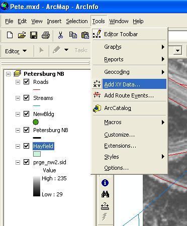
212 6-16

213 3. In the Add XY Data dialog that opens, navigate to the \nps_agis9\module6\data\pete\ folder and select the Arch.dbf file. Click Add. 4. If you click the dropdown arrow for X Field: or Y Field:, you will see that this table contains three fields: SITE_NO, X, and Y. The X coordinate data are stored in the X field and the Y coordinate data are stored in the Y field. Make sure that these fields are specified in the appropriate windows. Click OK. 5. A new Arch Events layer is added to the Table of Contents. Right-click on the layer and choose Zoom to Layer. 6. Click on the point symbol for the Arch Events layer in the Table of Contents and use the Symbol Selector to increase the point size to 8 and change the symbol color to a bright color. Click OK to apply the changes. 6-17

214 Create a Layer File (.lyr) from a Point Layer based on Tabular X/Y Data When you create a point layer from tabular X/Y data, it is often a good idea to save the layer as a layer (*.lyr) file for future use, as follows. 1. Right-click on the Arch Events layer name in the Table of Contents and choose Save As Layer File. 2. Save the Arch Events layer in the \nps_agis9\module6\data\pete folder. Click Save. 3. Now, save the map document as Pete2.mxd. From the File menu, select Save As, type Pete2.mxd for File Name:, and click Save to finish. You can use Pete2.mxd to complete the exercise at the end of this module. 4. Close ArcMap. Project Data On-the-Fly ArcMap can perform what is commonly known as on-the-fly projection. This means that ArcMap can display data stored in one projection as if it were in another projection. The actual data is not altered. This is explained in detail below. 1. Launch ArcMap and open the...\nps_agis9\module6\projection.mxd map document file. Notice that you can see elements from all three data layers in the view. 2. Select the View menu, and choose Data Frame Properties. 3. Choose the Coordinate System tab. Notice that the Current coordinate system is defined as NAD_1983_UTM_Zone_18N. 4. Click on Clear and then OK to close the Data Frame Properties window. 5. Notice that the LCS layer is no longer visible in the map display. 6. In the Table of Contents right-click on Park Boundary, and choose Properties. 7. In the Layer Properties window select the Source tab. 8. Under Data Source notice that the coordinate system is defined as NAD_1983_UTM_Zone_18N, which means this layer is stored in UTM, zone 18, NAD83 coordinates the same coordinate system that the data frame was in until you cleared it in Step

215 9. Click OK to close the window. 10. Repeat these steps with the LCS layer (starting at Step 6). Notice that this layer s coordinate system is defined as GCS_North_American_1983, which means it is stored in latitude/longitude, which are three-dimensional, un-projected coordinates. 11. Click OK to close the window. 12. Right-click on the LCS layer again, and select Zoom to Layer. Notice that there are now several red polygons in the view, but that the Park Boundary and image layers can t be seen. This is because they are stored in a different coordinate system, and are therefore displayed a long way off screen. (At this point ArcGIS is treating all the layers as if they were in the same coordinate system. But since the X and Y values in the two coordinate systems are nowhere close to being the same, the data layers display a long way apart.) To view these layers together, you will need to define the Data Frame s coordinate system as NAD_1983_UTM_Zone_18N that is, undo what you did in Step 4 or as some new coordinate system. You ll do the latter. 13. Right-click on Layers and choose Properties to open the Data Frame Properties window. 14. Choose the Coordinate System tab. 15. Under Select a coordinate system:, click on the Predefined folder, then click on the Projected Coordinate Systems folder, then on State Plane, and finally on NAD Scroll down to NAD 1983 StatePlane Virginia South FIPS 4502, and select it. 17. Click OK. You might not see much in the map display, but don t alter it. 18. Go to the View menu, and choose Bookmarks (you may remember from module 4, a bookmark stores a spatial extent that you can go back to later). In the fly-out menu choose South Zone. This takes you to a predefined spatial extent. You should now see part of the image and park boundary, along with several red polygons for the LCS layer. 19. Zoom in on the LCS polygons, and turn the layer off and on to verify that they are registered correctly to the image layer. 20. Close projection.mxd without saving the changes. 6-19

216 Module 6 Exercise Take a little time to explore different drawing and editing functions available in ArcMap. There are several menu items, buttons, and features that were not examined in this module that may be important to you in your work. Use the Petersburg image and the knowledge you have just acquired to digitize the fields, create a point shapefile of buildings, and edit the roads layer within the shaded area shown below. You may reuse the point and polygon layers that you created in this module. 1. Digitize the large field above the industrial complex, excluding the parking lot. 2. Correct the U shaped road in the industrial complex to follow the roads in the image. 3. Using the image as a guide, extend the U shaped road from the bottom right (southeast) corner to the southeast and then north-northeast to its end point. 4. Add points to the New Bldgs layer to represent the buildings in the industrial complex. 6-20

217 Module 7

218 Introduction to ArcGIS for Module 7: Geoprocessing Geoprocessing in ArcMap 9.x allows you to analyze and combine layers in different ways based on the spatial relationships among features. Spatial analysis tools available in ArcMap and ArcCatalog are accessed through the ArcToolbox Window. These include the Geoprocessing Tools, Clip, Dissolve, Intersect, Merge, and Union. Clip reduces the spatial extent of one layer based on the extent of another. Dissolve aggregates features in a single layer that have the same attribute values. Intersect finds those features falling within the spatial extent common to two layers. Merge combines two or more adjacent layers into a single layer. Union combines two polygon layers. The above geoprocessing tools are included in ArcGIS 9.1 out-of-the-box, however they are not in version 9.0; rather they are located in the Geoprocessing Wizard Tools toolbox which can be downloaded from: Once downloaded you can add it to the ArcToolbox window. Refer to the ArcGIS Desktop Help topic Adding toolboxes for more information. The Buffer Tool allows you to find features that are within a specified distance of other features. You can buffer features at a specific distance or use an attribute value to create variable width buffers. In addition, a Spatial Join is used to join the attributes of features in one layer to the features in another layer based on spatial relationship. Similar to Selection by Location, you can perform spatial joins based on containment, distance, and intersection relationships. All of the spatial data analysis operations introduced in this module create new spatial data sets from existing ones. Module Objectives At the conclusion of this module, you will be able to: Merge two shapefile layers into one layer Buffer a shapefile layer to create a new shapefile 7-1

219 Introduction to ArcGIS for Clip one shapefile layer with another shapefile layer Perform a spatial join Create summary tables Dissolve boundaries between adjacent areas within one shapefile based on attributes Overlay two shapefile layers using union or intersect ArcGIS 9.1 Geoprocessing Tools THIS IS VERY IMPORTANT Note that the exercises contained in this module, as well as subsequent exercises throughout the remainder of the course, were written for use with ArcGIS 9.0. For users running ArcGIS 9.1 there is no Geoprocessing Wizard Tools toolbox, thus the geoprocessing tools will be found in different locations within ArcToolbox than the exercises indicate as follows: Clip: Analysis Tools > Extract Dissolve: Data Management Tools > Generalization Intersect: Analysis Tools > Overlay Merge: Data Management Tools > General Union: Analysis Tools > Overlay Also note that the windows and options for these tools may also differ slightly from those indicated in the exercises. Application Scenario In this module, you will perform analyses to address the following hypothetical application scenario: The Resource Management staff for Shenandoah National Park (SHEN) needs to monitor raccoons and would like to find the best places in the park to observe them. Using the park s GIS streams and land cover data for the Southern District as a model, you will locate the best areas to observe raccoons. Based on previous field research, raccoons seem to gather food within 66 meters of streams (i.e., within riparian areas). However, the land cover type in which raccoons are most likely to be seen is unknown. Therefore, Resource Management staff wants to know the acreage of each forest cover type within 66 meters of a stream. In addition, they want to know the number of previous raccoon observations in each cover type within riparian areas. 7-2

220 Introduction to ArcGIS for Map Document Setup 1. Launch ArcMap with a new empty map. 2. From the File menu, select Save As; navigate to the \nps_agis9\module7 folder; and save the map document as geoprocessing.mxd. 3. In the Table of Contents right-click the Layers data frame name and click Properties in the context menu that appears. 4. Click the General tab and enter the following Name for the data frame: SHEN Raccoon Sightings. 5. Set both Map Units and Display Units to Meters. 6. The Data Frame Properties dialog should look like this: 7. Click OK. 7-3

221 Introduction to ArcGIS for 8. Save the map document. (Click the File menu item, then click Save or click the Save button on the standard toolbar.) Note: Save the Map Document often throughout this exercise. 9. Using the Add Data button navigate to the \nps_agis9\module7\data\shen folder and add the following data layers to the SHEN Raccoon Sightings data frame (you may need to connect to the module7 folder using the Connect to Folder button): for_cov.shp (forest cover) per_strms.shp (perennial streams) pk_bound.shp (park boundary) raccoon.shp (raccoon sightings) 10. Using the Add Data button, add the following layer for which a coordinate system has not been defined: int_strms.shp (intermittent streams) Click OK if One or more layers are missing spatial reference information. Data from those layers cannot be projected is displayed. You re going to enter that information for that layer now. 11. Before you can define the coordinate system for a layer in the current map document, geoprocessing.mxd, you must remove the layer and save the ArcMap document. Rightclick on the int_strms layer and select Remove. Save map document changes by clicking on the Save button. (You may also need to close the ArcMap window, but try steps first. If it doesn t work, close ArcMap and then perform steps 12-14, then reopen ArcMap and the geoprocessing.mxd map document.) 12. Open ArcCatalog and navigate to the \nps_agis9\module7\data\shen folder. Rightclick on the int_strms.shp layer and select Properties. Click on the Fields tab and then on the grey box to the left of the Shape field name. A Field Properties box appears below. The last entry should read Spatial Reference and Unknown. Click on the box with the ellipsis ( ) in the lower right corner. This opens the Spatial Reference Properties window. You ve used this before to import a coordinate system. Now, instead you ll select a predefined coordinate system. Click on the Select button. 13. In the window that opens navigate to Projected Coordinate Systems > Utm > Nad 1927, select NAD 1927 UTM Zone 17N.prj, and click Add. 7-4

222 Introduction to ArcGIS for 14. Click OK to close the Spatial Reference Properties window, then click OK to close the Shapefile Properties window. The coordinate system has now been defined. 15. In ArcMap, using the Add Data button navigate to the \nps_agis9\module7\data\shen folder and add the int_strms layer back into the map document. This time you should not receive the message regarding the layer missing spatial reference information. 16. Arrange the layers in the Table of Contents as in the following graphic: 17. Save the map document! Merge Two Data Layers Now, you will merge the perennial streams layer with the intermittent streams layer. 1. From the Window menu select ArcToolbox, or click on the Show/Hide ArcToolbox Window button on the Standard toolbar. 2. In the ArcToolbox window, click on the plus symbol (+) to the left of the Geoprocessing Wizard Tools to expand the toolbox and view the tools it contains, then double-click on Merge to open the Merge window. You may want to expand the Merge window to view all the options available. 3. From the Input Features dropdown list select per_strms, then int_strms. For Output feature class location browse to and select the location where the Shenandoah data is stored, \nps_agis9\module7\data\shen\. Under Name of the output feature class type in shen_strms.shp you may need to scroll down to see all available options. For Feature class(es) that define the output fields (optional) select per_strms, then click on the icon next to Spatial Reference (optional). With the Coordinate System tab selected, click on Import, navigate to \nps_agis9\module7\data\shen\, and select per_strms.shp. Click OK in the Spatial Reference Properties box and in the Merge 7-5

223 Introduction to ArcGIS for window. Once the merge is complete click Close in the Merge dialog, and the new shen_strms layer will be added to your map document, geoprocessing.mxd. 4. Verify that shen_strms contains the contents of the two other stream files. An easy way to do this is to thicken the lines for the two original files to a width of 2, then make the thinner line sit on top and make it a brightly contrasting color, for example bright yellow. 5. Turn off the per_strm and int_strm layers. Or, you may delete the per_strm and int_strm layers by right-clicking on the layer name in the Table of Contents and selecting Remove from the context menu. 6. Save the map document! Buffer a Layer The next step in your analysis involves creating a 66 meter buffer around all of the streams in the park. 7-6

224 Introduction to ArcGIS for 1. In the ArcToolbox window, expand Analysis Tools, then Proximity, and then doubleclick Buffer to open the Buffer window. As with the Merge tool, you may want to expand the Buffer window to view all the options available. 2. From the Input Features dropdown list select shen_strms. In the Output Feature Class box, navigate to the \nps_agis9\module7\data\shen\ folder, and enter buff66_strms.shp as the file name. 3. In the Linear Unit box, enter 66 and set distance units to Meters. 4. Use the Show Help option to explore what the Side Type and End Type options permit. In this instance, leave both at the default (Side Type = Full, End Type = Round). 5. In the Dissolve Type (optional) box, select the All option. Your window should now look like this: 7-7

225 Introduction to ArcGIS for 6. Click OK in the Buffer window and then Close in the Buffer dialog. Notice that the buff66_strms layer is added to the map s data frame. 7. Move your two new layers, shen_strms and buff66_strms, to appropriate positions in the Table of Contents. You may want to zoom in to see the results in more detail, then perform a Zoom to Full Extent. 8. Save the map document! Clip a Layer In the next series of steps, you will use a clip operation to create a forest cover layer in which the forest cover polygons are entirely within the 66-meter stream buffer you just created. In effect, you will clip out portions of forest cover polygons that fall outside the stream buffer. 1. In the ArcToolBox window, from the Geoprocessing Wizard Tools double-click on Clip to open the Clip window. 2. From the Input Features dropdown list select for_cov. 3. From the Clip Features dropdown list select buff66_strms. 4. In the Output Feature Class box, navigate to the \nps_agis9\module7\data\shen\ folder, enter riparian.shp as the file name, and click Save. 5. The Clip dialog should look like this: 6. Click OK and then Close. Notice that the riparian layer is added to the map s data frame. 7-8

226 Introduction to ArcGIS for 7. Use the Identify tool or open the attribute table to examine some of the attributes of the riparian layer features. 8. Change the symbology of the new layers (shen_strms, buf66_strms, and riparian) as desired, as well as their order in the Table of Contents. 9. Save the map document! Update Area and Perimeter Field Values THIS IS VERY IMPORTANT When you use the Geoprocessing Wizard operations, such as clipping one layer with another, and you save the output as a shapefile, the area, perimeter, and/or length of the features in the new shapefile are not calculated automatically. If you open the attribute table for your new riparian data layer, you will see that there are values in the AREA and PERIMETER fields, however, many of these values ARE NOT CORRECT. Since the input layer, for_cov, had AREA and PERIMETER field values, these attributes are carried over into the output layer, (riparian), but the values are not updated to reflect the new feature geometry. The following example will show you how to update the AREA and PERIMETER values for the riparian layer. (See Module 5 if you need to review how to calculate field values.) 1. Open the attribute table for the riparian layer. (In the Table of Contents, right-click the riparian layer, and click Open Attribute Table.) 2. On the standard toolbar, click the Editor toolbar button to open the Editor toolbar. 3. From the Editor toolbar dropdown list click on Start Editing. 4. As in Module 6, if the Starting To Edit In a Different Coordinate System dialog appears, click the Start Editing button. Note: it is not recommended that you alter the geometric attributes (area, length, perimeter, etc.) or the shape or location of spatial features in a layer that are being projected on-the-fly (covered at the end of this module)! The riparian layer is not being projected on-the-fly, so it is safe to edit it even if you receive the warning Starting to Edit In a Different Coordinate System, but it is important to be aware of this in other instances. 5. In the Attributes of riparian table, right-click on the AREA field heading and click Calculate Values. 6. In the Field Calculator, check the Advanced option. 7. The following Visual Basic (VB) statement needs to be entered in the Pre-Logic VBA Script Code box, but you ll copy it from ArcGIS help rather than typing it. Click on the 7-9

227 Introduction to ArcGIS for Help button in the Field Calculator window, and scroll down about one third of the way until you find the following text: Dim Output as double Dim parea as Iarea Set parea = [shape] Output = parea.area 8. Highlight this text in the help document and press Ctrl + C on the keyboard to copy it into the clipboard. Click the pointer in the Pre-Logic VBA Script Code box so the cursor appears and press Ctrl + V to paste the text from the help document. 9. In the AREA = box (at the bottom of the window) type Output. 10. The Field Calculator dialog should now look like this: 11. Click OK. The AREA field values are updated. Next, you will update the attributes values for the PERIMETER field. 12. In the Attributes of riparian table, Right-click on the PERIMETER field heading and click Calculate Values. 13. In the Field Calculator, copy and paste the following VB statement from the Help window (as you did before with the area update, but refer to calculate Length or Perimeter) into the Pre-Logic VBA Script Code box: Dim Output as double 7-10

228 Introduction to ArcGIS for Dim pcurve as ICurve Set pcurve = [shape] Output = pcurve.length 14. In the PERIMETER = box, type Output. 15. The Field Calculator dialog should look like this: 16. Click OK. The PERIMETER field values are updated. 17. From the Editor toolbar dropdown list click Stop Editing. 18. Click Yes when Do you want to save your edits? is prompted. This saves the newly calculated values for the AREA and PERIMETER fields to the Attributes of riparian table. Changes are not saved until you Save the edits. 19. Close the Attributes of riparian table. 20. Save the map document! 7-11

229 Introduction to ArcGIS for Spatial Join With a spatial join, you can find features that are closest to other features, features that are inside other features, and features that intersect other features. Similar to joining two tables by matching attribute values in a key field (Module 5), a spatial join appends the attributes of features in one layer to the features in another layer based on criteria that you specify. A spatial join provides a permanent association between two layers because it creates a new layer containing attributes from both input layers. In this section you will join the attributes of riparian layer polygons to the attributes of the raccoon layer (point). The end result will be a point layer (raccoon sighting locations) in which each point has the attributes of the parent raccoon layer and the attributes of the riparian polygon in which it is located. This is similar to a point in polygon overlay. 1. In the Table of Contents, right-click the raccoon layer name; and then from Joins and Relates, click Join. 2. From the first dropdown list in the Join Data dialog, What do you want to join to this layer, select Join data from another layer based on spatial location. 3. From the Choose the layer to join to this layer : dropdown list select the riparian layer. 4. Item No. 2 in the Join Data dialog now indicates that You are joining Polygons to Points. 5. Under Each point will be given all the attributes of the polygon that: select it falls inside. 6. In the Specify output shapefile or feature class for this new layer: box, type \nps_agis9\module7\data\shen\join_raccoon.shp. 7-12

230 Introduction to ArcGIS for 7. The Join Data dialog should look like this: 8. Click OK. The new layer, join_raccoon, is added to the Table of Contents. 9. Open the attribute table for the new join_raccoon layer. If necessary, scroll to the right to see that forest cover attributes (AREA, PERIMETER, FOR_COV, FOR_COV_ID, and FOREST_TYP) are appended to each raccoon sighting record, except the last one. 10. Save the map document. Create a Summary Table 1. In the Attributes of join_raccoon table, right-click on the FOREST_TYP field heading and click Summarize from the menu options. 2. The Summarize dialog opens. From the Select a field to summarize dropdown list, select FOREST_TYP. 7-13

231 Introduction to ArcGIS for 3. In the Choose one or more summary statistics to be included in the output table, click on AREA and check the box next to Sum. 4. In the Specify output table box enter \nps_agis9\module7\data\shen\analysis.dbf. 5. The Summarize dialog should now look like this: 6. Click OK. 7. Click Yes when prompted with Do you want to add the result table in the map?. 8. Close the Attributes of join_raccoon table. 9. Open the analysis table by right-clicking on it in the Table of Contents and selecting Open. 10. Examine the contents of the analysis table. Notice it contains the total area (Sum_AREA) and total number of table records (i.e., raccoon sightings) per forest type (Count_FOREST_TYP) for each unique forest type in the FOREST_TYP field. How many raccoon sightings have occurred in areas of Yellow Poplar? (13). 7-14